Project Description
Create a habitat suitability model for Juniperus scopulorum Sargent, a tree native to the Rocky Mounatin Region of North America. This habitat suitability model will focus on creating a modular, reproducible workflow. While climate change has changed or taken away suitable habitats for some plant species, the Rocky Mountain Juniper has remained stable and is even expaning habitat areas eastward (Hanberry, B., 2022). However, this is at the expense of other ecosystems. Some climate change scenarios predict up to 90% loss of suitable habitats native grass species like Sorghastrum nutans (Kane et al., 2017). So, when thinking about grassland restoration, the effects of climate change and expanding species like Juniperus scopulorum Sargent must be taken into consideration for long-term viability of other plant species and ecosystems. This project will choose two study areas - National Grasslands, one in southern Colorado - Comanche National Grassland, and one in Nothern Colorado - Pawnee National Grassland. Both of these National Grasslands are in the Eastern Plains of Colorado which are to the east of the Rocky Mountains. The model used will be based on combining multiple data layers related to soil, topography, and climate (as raster layers) within the study area envelope (the two grasslands chosen).
One variable related to soil is chosen (from POLARIS dataset):
- pH (soil pH in H2O)
Elevation from the SRTM:
- Slope
Two climate scenarios are chosen from the climate model CCSM4 (NCAR): (precipitation, monthly)
Historical
rcm85 (worst case scenario)
Citations
Hanberry, B (2022). Westward Expansion by Juniperus virginiana of the Eastern United States and Intersection with Western Juniperus Species in a Novel Assemblage, volume 13, ISSN 999-4907, doi 10.3390/f13010101, number 1, journal - Forests, publisher - MDPI AG, year- 2022, month - jan, pages- 101.
Kane K, Debinski DM, Anderson C, Scasta JD, Engle DM and Miller JR (2017) Using Regional Climate Projections to Guide Grassland Community Restoration in the Face of Climate Change. Front. Plant Sci. 8:730. doi: 10.3389/fpls.2017.00730
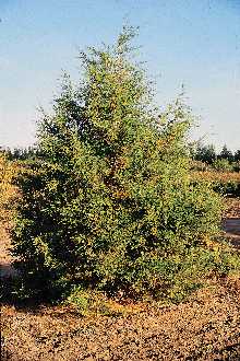
Plant Species Description
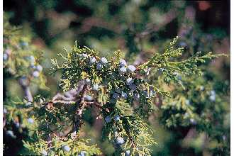
Juniperus scopulorum Sargent, also known as Rocky Mountain Juniper Tree, is a coniferous tree that slowly grows to about 20 feet at 20 years but can grow up to 50 feet mature (Characteristics of Juniperus scopulorum Sarg., USDA, NRCS). It also has a long life span with high drought tolerance which works to its favor in semi-airid climates like that of the Eastern Colorado Plains (Characteristics of Juniperus scopulorum Sarg., USDA, NRCS). It is native to North America throughout the Rocky Mountain region between British Colombia and Alberta, Canada all the way south through the continental U.S. to the four corners states and east through some of the Great Plains states (Stevens, 2008). The Rocky Mountain juniper grows best below elevations of 7,500 feet, but typically between 5,000 and 7,500 feet (Plant Materials Program, 2002). While the Rocky Mountain juniper is frequently used as an ornamental tree or shrub tree in wildlife plantings and shelterbelts, it is also used by a range of birds and mammals for its ground cover or nesting materials. The Rocky Mountain junipers' berries also provide an important part of both bird and mammal diets. Additionaly, First Peoples have used this berries from this juniper for tea and other applications for medicinal purposes (Stevens, 2008). Some potential problems or concerns about this tree/shrub tree are that it carries cedar-apple rust disease which is not harmful to itself but is harmful to other tree species (Plant Materials Program, 2002). Beyond diseases, the Rocky Mountain juniper increases are "at the expense of other ecosystems, such as shrublands, grasslands, riparian forests, and open pine and oak forests, with consequent impacts on plant and wildlife species that flourish in open or unique ecosystems" (Hanberry, B., 2022).
This species was chosen because of its prevelance in both the Pawnee National Grassland and the Comanche National Grassland. For the Pawnee National Grassland, the 'General Technical Report' from the USDA, Forest Service on Vascular Plant Species of the Pawnee National Grassland states that the Juniperus scopulorum Sargent occurs in the cliffs and ravines of this National Grassland (Hazlett, 1998). Similarly in the Comanche National Grassland, this same type of technical report states that Juniperus scopulorum Sargent occurs in all 3 counties (Baca, Otero, and Las Animas Counties) that this grassland is in, which also grow in "shaded rocky canyons and ravines" and "Rocky: exposed limestone/shale barrens" (Hazlett, 2004). Because this species is expanding habitats, I am curious to see what the outcome of the habitat suitability model will be. This project could be done with any plant species of choice and could even be adapted to animal habitat suitability, but using other datasets and variables that would pertain to that species or locations of study areas chosen.
Considering its growth conditions, Juniperus scopulorum Sargent has optimal pH values between 8.5 (max) and 5 (min), and annual precipitation between 26 inches and 9 inches (66cm - 23cm) (Characteristics of Juniperus scopulorum Sarg., USDA, NRCS).Root depths at a minimum are 9 inches (23cm) (Characteristics of Juniperus scopulorum Sarg., USDA, NRCS). While there are other factors that could be taken into consideration for growth, those are the two variables that will be chosen for this project. These variables will be further discussed in the 'Data Description' section. To look at other growth condition factors as well as additional information about Juniperus scopulorum Sargent, please visit Natural Resources Conservation Service - USDA, Plant Profile Characteristics for Juniperus scopulorum Sarg..
Citations
Characteristics of Juniperus scopulorum Sarg. Rocky Mountain juniper. U.S. Department of Agriculture, Natural Rescources Conservation Service, Accessed 30 November, 2024.
Hanberry, B (2022). Westward Expansion by Juniperus virginiana of the Eastern United States and Intersection with Western Juniperus Species in a Novel Assemblage, volume 13, ISSN 999-4907, DOI 10.3390/f13010101, number 1, journal - Forests, publisher - MDPI AG, year- 2022, month - jan, pages- 101.
Stevens, Michelle (edited 2008). Plant Guide for Rocky Mountain Juniper. United States Department of Agriculture,Natural Resource Conservation Service, National Plant Data Center.
Plant Materials Program (edited 2002). Plant Fact Sheet for Rocky Mountain Juniper. United States Department of Agriculture,Natural Resource Conservation Service.
Hazlett, Donald L. 1998. Vascular plant species of the Pawnee National Grassland. General Technical Report RMRS-GTR-17. Fort Collins, CO: U.S. Department of Agriculture, Forest Service, Rocky Mountain Research Station. 26 p. (https://www.fs.usda.gov/rm/pubs/rmrs_gtr017.pdf).
Hazlett, Donald L. 2004. Vascular plant species of the Comanche National Grassland in southeastern Colorado. Gen. Tech. Rep. RMRS-GTR-130. Fort Collins, CO: U.S. Department of Agriculture, Forest Service, Rocky Mountain Research Station. 36 p. (https://www.fs.usda.gov/rm/pubs/rmrs_gtr130.pdf)
Site Descriptions
Land Acknowledgement: First Peoples and Indigenous Peoples are the original stewards of the land taken before, during, and beyond colonialism in the Americas. Much of recorded history has prioritized Euro American perspectives and experiences that have misrepresented, excluded, and erased Black, Indigenous, and People of Color perspectives and experiences (History Colorado, Grounding Virtues). First People's and Indigenous People's stewardship and connection to this land must be honored and respected.
Please read the land acknowledgement above the map before continuing reading, it is imperative to naming and confronting racialized systems that dominate history and our current era.
Two study areas were chosen from the U.S. National Grassland Units. Both of these grasslands are in Colorado, one in nothern Colorado and one in southern Colorado. I chose these two study areas specifically because I wanted to see if there was a difference between the northern grassland (Pawnee) and the southern grassland (Comanche) in terms of habitat suitability. A possible disadvantage to choosing two grasslands that are relatively close to one another is that the model outcomes showing a more suitable habitat in a certain study area, may not be noticeable. An advantage may be providing model outcomes within a singular unit of a state or Colorado Eastern Plains region, is providing insight for that area.
The two grasslands are similar in that they are split geographically in two units or areas, however the Comanche is about twice the size of the Pawnee National Grassland.
Comanche National Grassland


The Comanche National Grassland "is named in honor of the Comanche tribe. The Comanche name is believed to be derived from Komontcia, a Ute word that means 'People Who Fight Us All the Time' (Pritzker 2000). This nickname, assigned by the Utes, reflects the Comanche reputation among other tribes and among pioneers as fierce fighters" (Hazlett, 2004, pg. 3). Between the 18th and 19th centuries there were many 'claims' to this land where the Comanche National Grassland currently is situated by absentee ownership of the U.S., France, and Mexico, but by 1853 the Comanche were 'asked' (forced) to sign a 'treaty', which ceded any remaining lands that were not previously ceded (taken)(Hazlett, 2004, pages 1-4). Thus the "remaining Comanche groups in southeastern Colorado had lost their homeland and lifestyle" (Hazlett, 2004, page 3).
After the Dust Bowl resulted in much abandoned farmland the "National Industrial Act and Emergency Relief Appropriations Act that passed Congress in 1933 and 1935 gave the Federal government the authority to purchase failed crop lands" (Wooster 1982). It wasn't until 1954 that "the administration of these lands was transferred to the USDA-Forest Service" (Hazlett, 2004, page 4). In 1960 the Comanche National Grassland was created to be managed by the USDA-Forest Service to conserve "the natural resources of grass, water and wildlife habitat(s)" and protect prehistoric and historic, cultural and natural assets ("Comanche National Grassland, USDA FS"). It consists of around 440,000 acres of discontinuous land that is located in the corner of southeastern Colorado ("Comanche National Grassland, USDA FS"). This grassland is situated between three different Colorado counties: Baca, Otero, and Las Animas and can be further identified as two distinct units the Carrizo Unit south and west of Springfield and the Timpas Unit south of La Junta" (Hazlett, 2004, page 4).
The Comanche National Grassland is within what most plant geographers classify as the 'North American Prairie Province' (Hazlett, 2004, page 5). Rockey Mountain junipers grow in 'rocky outcrops' which "are areas within the open steppe, such as hilltops, where erosion has exposed a rocky surface or barren. A “barren” is defined here, in a broad sense, as a sparsely vegetated exposed bedrock of shale, shale-derived soils, chalk, or limestone soilswith microorganisms in a calcite matrix (Kelso et al., 2003),(Hazlett, 2004, page 8 and 17). They also grow in the Comanche National Grassland in 'shaded rock canyons and ravines' which are characterized as "the steep, rugged relief areas that comprise the rocky cliffs, rock slicks, and shaded ledges in the major canyons... Included here are hills with large boulders and steep ridges... The greater water availability along cliff faces is complemented by less evaporation due to greater amounts of shade. This is a habitat of deep water percolation and occasional shade" (Hazlett, 2004, page 8 and 17). Due to the vast expanse of land the Comanche National Grassland occupies (over 100 miles from one end to the other) the "Annual rainfall amounts on the Comanche National Grassland have a high degree of spatial and temporal variation." (Hazlett, 2004, pages 4-5). The closest weather center, Western Regional Climate Center (WRCC), reports a 55-year annual average as 11.5 inches ; however, this climate center is 4 miles away from La Junta, which is north of Vogel Canyon (see map above, La Junta would be off the map to the north of Vogel Canyon) (Hazlett, 2004, pages 4-5). So, that percipitation number would not be accurate or reflective of all of this National Grassland due to its size.
The Vascular plant species of the Comanche National Grassland in southeastern Colorado by Donald Hazlett, 2004, was very comprehensive not only of vegetation, but also history, geology, and climate and should be read if interested in more in depth context information than can be provided here.
Pawnee National Grassland


There is a lack of information available on this particular grassland as it relates to First Peoples, and most context information I am finding about the history of this grassland starts with settlers or pioneers 'settling' the land which feeds the Euro American perspective on history and excluding Indigenous perspectives and experiences of this land. What little information I did find was in someone's blog stating that "these lands were the home of the Arapaho and Cheyenne, who were forcibly removed in the 1880s to allow white settlers to establish homesteads and farm the land" (Diana 2021). However, there was no source given as to where this blogger found that information. I acknowledge that much more research is needed for the historic and cultural context that does not start with pioneers.
That being said, settlers in the mid 19th century used this land for cow grazing due to the aird nature of the land being difficult to grow crops (Rhoads, D. and L.). Later in the late 19th century through the early 20th century there were waves of newcomers and continued use of land for grazing, but similar to the Comanche National Grassland the after effects of the Dust Bowl lead to the U.S. Forest Service mangaing the area in 1954 then getting permanent control in 1960 (Rhoads, D. and L.). The Pawnee National Grassland differs from the Comanche in that it has over 200 avtive oil and gas leases on the grassland that are managed by the Bureau of Land Management, and the U.S. Forest Service "specifies the revegetation procedures to be followed by the private operators while conducting their exploration, drilling and production activities" (Rhoads, D. and L.). This land is about 10% of the Pawnee National Grassland and is labeled (CPER - Central Plains Experimental Range) on the map above (Hazlett, 1998, page 2). It should be noted that the data used for the study area - U.S. National Grassland Units, include this private land and that should be kept in mind with any analyses.
The Pawnee National Grassland consists of around 193,000 acres of discontinuous land (less than half the size of the Comanche National Grassland) that is located in northeastern Colorado, Weld County, on the border of Wyoming (Hazlett, 1998, pages 1-2). This grassland is within the Central Shortgrass Prairie Ecoregion and "geomorphic sections of the Great Plains province known as the High Plains and the Colorado Piedmont (Trimble 1993)" (Hazlett, 1998, pages 3-4). Rocky Mountain junipers grow in similar areas in this grassland as they do in the Comanche National Grassland - in cliffs and ravines (Hazlett, 1998, page 7). The climate here is affected by "continentality, air masses, and mountain barrier" of the Rocky Mountains which block marine polar air masses from the west contributing to the drier conditions on the Great Plains (Hazlett, 1998, page 1). The 21-year average annual rainfall, measured between 1969-1989, was 12.6 inches which is similar to the annual average from the Comanche National Grassland (11.5 inches) (Hazlett, 1998, page 1). However, this data is out of date considering the current increased impact of climate change.
The Vascular plant species of the Pawnee National Grassland
by Donald Hazlett, 1998, was also comprehensive not only of vegetation, but also
geology, soils, and climate and should be read if interested in more in depth
context information than can be provided hhere. While this publication is missing
the historic context related to the site, unlike his later report on the Comanche
National Grassland, it is still very detailed and worth the read!
Citations
History Colorado. "Grounding Virtues" from History Colorado Anti-Racism Work (https://www.historycolorado.org/sites/default/files/media/document/2020/Anti-Racism_Grounding_Virtues.pdf).
Pritzker, B.M. 2000. A Native American encyclopedia: history, culture and peoples. New York, NY: Oxford University Press. (https://archive.org/details/nativeamericanen0000prit/page/n9/mode/2up)
Hazlett, Donald L. 2004. Vascular plant species of the Comanche National Grassland in southeastern Colorado. Gen. Tech. Rep. RMRS-GTR-130. Fort Collins, CO: U.S. Department of Agriculture, Forest Service, Rocky Mountain Research Station. 36 p. (https://www.fs.usda.gov/rm/pubs/rmrs_gtr130.pdf).
Wooster, D. 1982. Dust Bowl: the southern plains in the 1930s. New York, NY: Oxford University Press, Inc. (https://global.oup.com/ushe/product/dust-bowl-9780195174885?cc=us&lang=en&)
Comanche National Grassland. U.S. Department of Agriculture, Forest Service. Accessed 30 November, 2024. (https://www.fs.usda.gov/recarea/psicc/recarea/?recid=12409)
Kelso, S.; Bower, N. W.; Heckmann, K. E.; Beardsley, P. M.; and Greve, D. G. 2003. Geobotany of the Niobrara chalk barrens in Colorado: a study of edaphic endemism. Western North American Naturalist 63(3): 299-313. (https://www.jstor.org/stable/41717298)
Diana, No last name given. Colorado Destinations: Pawnee National Grassland. Handstands Around the World. June 21, 2021. (https://handstandsaroundtheworld.blog/2021/06/21/colorado-destinations-pawnee-national-grassland/)
Rhoads, Dorothy and Lee, former volunteers for the U.S. Forest Service. Pawnee National Grassland History. U.S. Department of Agriculture, Forest Service. Accessed 1 December, 2024. (https://www.fs.usda.gov/detail/arp/learning/history-culture/?cid=fsm91_058308)
Hazlett, Donald L. 1998. Vascular plant species of the Pawnee National Grassland. General Technical Report RMRS-GTR-17. Fort Collins, CO: U.S. Department of Agriculture, Forest Service, Rocky Mountain Research Station. 26 p. (https://www.fs.usda.gov/rm/pubs/rmrs_gtr017.pdf).
Trimble, D.E. 1993. The geologic history of the Great Plains. Reprint with minor revisions of Geological Survey Bulletin 1493. Theodore Roosevelt Nature and History Association, Medora, ND. 54 pp. (https://pubs.usgs.gov/bul/1493/report.pdf)
Data Descriptions
Administrative Boundaries: USFS National Grassland Units (used for study sites)
The USFS (United States Forest Service) National Grassland Units is a dataset of administrative boundaries of National Grasslands. This is just one feature layer that the USFS Geospatial Data Discovery website has to offer. There are many other types of data topics such as forest management, ecosystems, hydrology, and more that can be further explored.The USFS Grassland Units feature layer, like the other data available on this webpage, was created by the USFS, an authoritative source, to provide geospatial data published by the agency. This particular layer is used in this project in order to provide the study area boundaries. Specific grassland boundaries can be selected from the layer, for this project the Comanche and Pawnee National Grasslands will be selected. This data is downloaded as a shapefile and the boundaries of the national grasslands will provide the base for the other data in this project (raster layers) to be built upon.
A disadvantage to using these boundaries are that the areas are typically discontinuous so it may potentially be difficult to visually see analyses on plots. Other shapfiles could also be used as boundaries like National Parks, Forests, or other defined units that match with the species chosen or goals of research.
The USFS Grassland Units data was created in 2017 and says that it is updated weekly but the last update was in 2022; however, the boundaries or land associated with these in theory wouldn't be drastically changing on a weekly or even monthly basis. This data is publically accessible and can be used under a CC0 1.0 License, which essentially means there is no copyright and permission is not needed to use it.
Soil Data: POLARIS soil properties database (variables related to soil)
The POLARIS database for soil properties is a database of a century of soil survey data that is on a server hosted by Duke University. However, while part of the data collected comes from soil surveys, this dataset fills in unsruveyed areas with a series of probabilities for what the soil type in a specific area is. This filling in helps create a continuous layer to work with and makes it easier to work with choosing a study area where not every 30m by 30m section was surveyed, and still able to use this data. For analysis it does need to be kept in mind that the filled areas may not be totally accurate, but they are a good estimate of what the soil type is. There are 13 soil property variables available, each with 5 statistics avaialble, at 6 different depth layers, then 1x1 degree tifs (Dr.Chaney). The README on this data set states an important notice about these tifs - "Due to file size constraints, the 1 arcsec database is split into 1x1 degree tiffs. Each variable/layer/statistic has its own virtual raster that acts as the "glue" of all the smaller 1x1 degree chunks. For more information on virtual rasters see https://www.gdal.org/gdal_vrttut.html" (POLARIS soil properties datbase). Besides the README there are helpful websites that give more information about this datset such as POLARIS – a probabilistic soil classification and property database over the contiguous United States at a 30-meter spatial resolution , Polaris 30m Probabilistic Soil Properties US, and Chaney et al..
An advantage of using this dataset is that it provides a "spatially continuous, internally consistent, and quantitative prediction of soil classification and property database with a high degree of granularity (30-meter) covering the entire contiguous United States" (Dr. Chaney). A disadvantage to this database would be that this is only for the contiguous United States (CONUS).
For this particular project, two variables are chosen, pH and theta_s which is saturated soil water content, m3/m3. These two variables were chosen because optimal levels or measurements of both were found for the Rocky Mountain Juniper. These two variables will use the mean statistic available at the 60-100cm depth (this relates to root depth of the plant species chosen). Mean is one of the easier statistics given to work with which is why it was chosen. The 60-100cm depth was chosen because the minimum root depth for the Rocky Mountain Juniper is 51cm which does fall in the 30-60cm depth, however because 51cm is the minimum and would fall in the latter part of that depth range, the range above this was chosen. Make sure to pay atttention to the depth being used which depends on the root depth of the plant species chosen. This dataset is in 30m resolution which is needed in order to harmonize the rasters.
This database is accessible and can be used under Creative Commons Attribution-NonCommercial 4.0 International License. The database can be accessed here - POLARIS soil properties database
Elevation Data: earthaccess API (elevation from the SRTM - used to calculate slope)
Earthaccess "is a python library to search for, and download or stream NASA Earth science data with just a few lines of code" (earthaccess API (description in User Guide)). This library is made available by the National Snow and Ice Data Center (NSIDC), with many contributors to this specific repository which is publically accessible. Earthaccess is a great contribution to open science efforts making it easier to access and download NASA datasets by "reducing barriers to cloud based analysis" (earthaccess API (description in User Guide)).
Earthaccess API (Application Programming Interface) is used in this project to access elevation data from the SRTM (Shuttle Radar Topography Mission) via an internet web interface. The earthaccess API bascially makes a request to this data repository and returns requested data per parameters given, in this case parameters will be set in order to access a subset of data for elevation. The SRTM data is data that has "been enhanced to fill areas of missing data (Void Filled) to provide more complete digital elevation data", otherwise there would be missing tiles in the data. This data is available at a 30 meter (1 arc second) resolution which is the same as the POLARIS data which is important. While there are a few data formats and file formats of the SRTM available, for this project the ____ data format is used, and the ____ file format. These are used because .....
SRTM data was collected via a satellite mission on the Endeavour in 2000 by NASA and NGA (National Geospatial-Intelligence Agency) to collect radar data to create the first near global set of land elevations (Earth Resources Observation and Science (EROS) Center). Because this data comes from authoritative sources it can be trusted to a degree, but will need to keep in mind that the void filled areas while "using interpolation algorithms in conjunction with other sources of elevation data", may not be 100% accurate. To learn more about the Shuttle Radar Topography Mission itself, as well as data and file formats of SRTM please vist USGS EROS Archive - Digital Elevation - Shuttle Radar Topography Mission (SRTM).
The earthaccess API is publically available and the SRTM data is open data as long as proper attribution is given to these sources. To preview the SRTM data visit Earth Explorer which can help with making sure data is available for a certain area in a certain time frame, etc. to set up parameters wanted when using the earthaccess API.
Climate Data: MACAv2 via THREDDS data server (climate scenarios)
Climate Projection Models are one way to guide restoration of many habitats in face of climate change. These projection models use outputs of Global Climate Models (GCM), which simulate the global and regional scale climate processes that have data collected from satellites, weather stations, oceanic buoys, and other methods. As part of the Climate Model Intercomparison Project phase 5 (CMIP5), data was drawn from over 40 GCM's from coutnries across the globe to analyze and compare these many GCM's (Taylor et al., 2012). This comparison allows for better understanding of climate change now/historically as well as in the future. However, one of the drawbacks of this being global data is that it has coarse resolution because of the scale, so an image or map using the data would appear like a pixelated photo of low resolution.
One way to try to combat this coarse resolution is to downscale this spatial data. MACA V2 (Multivariate Adaptive Constructed Analogs, version 2) does just that (Abatzoglou and Brown, 2012). Using statistical operations (find more information here) , that result in a 4km resolution which produces a higher resolution image. It should be noted that MACA V2 is only for CONUS, a similar type of dataset may heve been done in other regions globally but that would need to be researched further if interested in a project location outside CONUS. This higher resolution will complement the other raster data being used in this project which is at a 30 meter resolution (POLARIS and SRTM). While 4km and 30m are upon face value are vastly different numbers, climate data represents broader atmospheric conditions across a larger area, while the soil data is at a 30m resolution due to the much higher variability in soil properties and elevation across smaller distances, making finer detail necessary to accurately capture local soil characteristics and elevation. Essentially, climate is more uniform over larger areas compared to soil and elevation which can change significantly within a short distance.
While there are benefits to downsizing, a disadvantage to it is that due to the statistical methods used, introduces uncertainty. This needs to be kept in mind, but the MACA V2 dataset is widely accepted by many institutions and organizations such as the U.S. Forest Service.
The THREDDS (Thematic Real-time Environmental Distributed Data Services) data server is a web server that can be used to access the MACA v2 dataset as well as other scientific datasets (Unidata, UCAR). This catalog of datasets, accepts a few different data formats including NetCDF, GRIB, and HDF. Because the data in the MACA V2 dataset is available in NetCDF as its original format, that will work for this project. The MACA V2 is also available as tabular data and GeoTIFF.
MACA V2 has 20 different climate models, each of these models can be found here. Each of these has 9 climate variables to choose from, the climate variable options can be found here. There are 3 climate scenarios available: actual/historic, intermediate, and worst case climate scenarios. Climate scenarios avilable here are either different time periods or different emissions scenarios. For this project, the climate model CCSM4 is chosen, then climate variable chosen is percipitation and the two temporal climate scenarios will be used. Two different time periods are chosen (actual/ historic - 'historical , and worst case scenario - rcm85), and this route was chosen because it will aid in the analysis of suitable habitats for the Rocky Mountatin Juniper in both of the study areas chosen (Comanche and Pawnee National Grasslands). Different time periods provide insight into the past as well as possible future scenarios and the two can be compared to look at the validity of the habitat suitability model to be created for this project (this will be further discussed in the next section). The MACA data can be downloaded as daily or monthly, and for the purposes of this project, monthly will suffice, the amount of data the daily dataset would have, is not necessary here.
The MACA V2 data is available under a Creative Commons CC0 1.0 Universal dedication license - the dataset was "created with funding from the US government and are in the public domain in the United States" () This data server can be accessed here, but there are many ways the data can be downloaded, please see MACA website.
Citations
USDA U.S. Forest Service - Geospatial Data Discovery, U.S. National Grassland Units. Published April 14, 2017. Last Update August 26, 2022.
Dr. Chaney, Nathaniel. POLARIS – a probabilistic soil classification and property database over the contiguous United States at a 30-meter spatial resolution. Duke Translation and Commercialization - Available Technoligies. (https://otc.duke.edu/technologies/polaris-a-probabilistic-soil-classification-and-property-database-over-the-contiguous-united-states-at-a-30-meter-spatial-resolution/#:~:text=The%20POLARIS%20soil%20series%20database,of%20the%20currently%20available%20database.)
Polaris 30m Probabilistic Soil Properties US. awesome-gee-community-catalog. (https://gee-community-catalog.org/projects/polaris/#data-characteristics).
Chaney, Nathaniel W., Budiman Minasny, Jonathan D. Herman, Travis W. Nauman, Colby W. Brungard, Cristine LS Morgan Alexander B. McBratney, Eric F. Wood, and Yohannes Yimam. "POLARIS soil properties: 30‐m probabilistic maps of soil properties over the contiguous United States." Water Resources Research 55, no. 4 (2019): 2916-2938.
POLARIS soil properties database. (http://hydrology.cee.duke.edu/POLARIS/PROPERTIES/v1.0/).
earthaccess API (description in User Guide). List of contributors available on Github. Accessed December 2, 2024. (https://earthaccess.readthedocs.io/en/latest/user-reference/api/api/).
Earth Resources Observation and Science (EROS) Center. USGS EROS Archive - Digital Elevation - Shuttle Radar Topography Mission (SRTM). June 29, 2018. (https://www.usgs.gov/centers/eros/science/usgs-eros-archive-digital-elevation-shuttle-radar-topography-mission-srtm).
Earth Explorer. USGS. (https://earthexplorer.usgs.gov/).
Taylor, K.E., R.J. Stouffer, G.A. Meehl: An Overview of CMIP5 and the experiment design. MS-D-11-00094.1, 2012.
Abatzoglou J.T. and Brown T.J. (2012). "A comparison of statistical downscaling methods suited for wildfire applications". International Journal of Climatology, doi: 10.1002/joc.2312. Funding agencies: Regional Approaches to Climate Change (REACCH), the Climate Impacts Research Consortium(CIRC) and the Northwest/SouthEast Climate Science Centers(NWCSC,SECSC).
Portier, Andrea, (NASA GSFC / SSAI). Shedding Light on the Future of Earth's Climate with NASA Data. August 24, 2021. (https://gpm.nasa.gov/applications/shedding-light-future-earths-climate-nasa-data#:~:text=%E2%80%9CNASA%20is%20a%20leader%20in,decisions%20that%20directly%20impact%20society).
Unidata, UCAR. THREDDS Data Server version 4.6 Documentation - THREDDS Data Server 4.6. Updated November 2018. (https://docs.unidata.ucar.edu/tds/4.6/adminguide/#:~:text=The%20THREDDS%20Data%20Server%20(TDS,other%20remote%20data%20access%20protocols).
MACA website - "CMIP5 GCMs" (list). (https://climate.northwestknowledge.net/MACA/GCMs.php).
MACA website - "MACA Downscaled Variables". (https://climate.northwestknowledge.net/MACA/MACAproducts.php)
Methods Description
With the goal of building a habitat suitability model, there are many steps that need to happen prior to being able to do that.
Define study area(s): Download the USFS National Grassland Units and select 1 or more grassland units.
- I chose Comanche and Pawnee Nation Grasslands as study sites. The USFS National Grassland Units are 'administrative boundaries' and this data is used to bound and crop the 3 sets of raster data being used in this project as well as provide boundaries when plots are created.
Fit a model:
a. For each grassland, download model variables as raster layers covering the study area envelope, including:
i. 1 soil variable from the POLARIS dataset
- I chose pH. Using this raster data will provide insight into this soil property in the study areas chosen.
ii. Elevation from the SRTM (use the earthaccess API)
- This will be used to calculate slope later. For the Rocky Mountain Juniper, they are frequently located in ravines, canyons, and rocky barrens, so they woulc be located in areas with steep slopes, or where are are drastic differences in slope.
iii. 1 climate variable from the MACAv2 THREDDS) data server. This project will compare two climate scenarios of choice (e.g. different time periods, different emission scenarios).
- I chose the CCSM4 climate model, using the precipitation variable, and two climate scenarios - historical and rcm85. The model was chosen to best match the resolution of the other raster data being used in this project and because NCAR is in Colorado and I think data from NCAR has been used in other projects I've done. The climate variable precipitation was chosen because optimal levels of it were found in researching the Rocky Mountatin Juniper. Those two climate scenarios were chosen because choosing one model as the actual/ historical scenario and comparing to a future scenario is helpful in evaluating if the model can make predictions that are more reliable (Global Percipitation Measuremet Mission, NASA).
b. Calculate at least one derived topographic variable (slope or aspect) to use in the model. Use the xarray-spatial library, and update or install this library if not already on machine being used. Note that calculated slope may not be correct if using a CRS with units of degrees; need to re-project into a projected coordinate system with units of meters, such as the appropriate UTM Zone.
- I am choosing slope for this project because it more closely relates to where the Rocky Mountain Juniper is found in the Comanche and Pawnee National Grasslands. It is found in ravines, canyons, and rocky barrens, so the slope would possibly provide more information in the habitat suitablity model.
c. Harmonize data - make sure that the grids for each of the layers match up. Check out the ds.rio.reproject_match() method from rioxarray.
- This step is very important. The model cannot be built if the different layers are off or on different grids; they have to relate to one another in order to do the raster math in the next step. The data will be harmonized to the lowest resolution raster of the group, higher resolution can be made into a lower resolution, but not vice versa. Although this may sound bad, most of the rasters chosen are around 1x1 degrees so there should in theory not be a huge depreciation in resolution.
Build habitat suitability model - use any model, so long as the choice of model is explained. However, if it is not clear how to proceed, building a fuzzy logic model (see below) is best. I will be doing a fuzzy logic model.
To train a fuzzy logic habitat suitability model:
- Use research done on the plant species chosen (Rocky Mountain Juniper), and find the optimal values for each variable being used (e.g. soil pH (5-8.5), slope (5,000-7,500ft elevation), and current climatological annual precipitation (9 inches - 26 inches, 228.6 - 660.4 mm). For each digital number in each raster, assign a value from 0 to 1 for how close that grid square is to the optimum range (1=optimal, 0=incompatible). Combine raster layers by multiplying them together (raster math). This will output a single suitability number for each square. Another option would be to apply a threshold to make the most suitable areas pop on the map created.
Present the results of the model in at least one figure for each grassland/climate scenario combination.
- The output raster from the fuzzy logic habitat suitability model will be used with the overlay of the boundaries of the study area. Multiple plots will be made to account for each grassland/climate 'scenario, so there should be 4 plots to finish the concluding thoughts.
The climate scenarios chosen, actual/historical and worst case scenario are particularly important in this habitat suitability model because if the model can't predict obeservations made in real life then it is less likely "that a climate model will be able to predict future changes in rainfall and its influence on other components such as soil moisture" (Global Percipitation Measuremet Mission, NASA).
Citations
Global Percipitation Measuremet Mission, NASA. How do we Predict Future Climate?. (https://gpm.nasa.gov/education/sites/default/files/lesson_plan_files/climate-package/Climate%20Models.pdf)
Wasser, Leah, Chris Holdgraf, Martha Morrissey. The Intermediate earth data science textbook course: Lesson 2. Subtract One Raster from Another and Export a New GeoTIFF in Open Source Python. (https://www.earthdatascience.org/courses/use-data-open-source-python/intro-raster-data-python/raster-data-processing/subtract-rasters-in-python/). DOI: https://doi.org/10.5281/zenodo.4683910. License: CC BY-SA 4.0.
# Prepare for download Part 1 of 1
## Import packages that will help with...

# Reproducible file paths
import os # Reproducible file paths
import pathlib # Find the home folder
from glob import glob  # returns list of paths
import zipfile # Work with zip files

# Find files by pattern
import matplotlib.pyplot as plt # Overlay pandas and xarry plots,Overlay raster and vector data
import rioxarray as rxr # Work with geospatial raster data


# Work with tabular, vector, and raster data
import cartopy.crs as ccrs # CRSs (Coordinate Reference Systems)
import geopandas as gpd # work with vector data
import hvplot.pandas # Interactive tabular and vector data
import hvplot.xarray # Interactive raster
from math import floor, ceil # working with bounds, floor rounds down ciel rounds up
import numpy as np # numerical computing
import pandas as pd # Group and aggregate
from rioxarray.merge import merge_arrays # Merge rasters
import xarray as xr # Adjust images
import xrspatial # calculate slope

# Access NASA data
import earthaccess # Access NASA data from the cloud
# Set Up Analysis Part 2 of 2

# Define and create the project data directory
habitat_suitability_data_dir = os.path.join(
    pathlib.Path.home(),
    'earth-analytics',
    'data',
    'habitat_suitability'
)
os.makedirs(habitat_suitability_data_dir, exist_ok=True)

# Call the data directory to check its location
habitat_suitability_data_dir
'/Users/briannagleason/earth-analytics/data/habitat_suitability'
# Download USFS National Grasslands Units Data Part 1 of 1

# Define info for USFS Grasslands download
usfs_grasslands_url = (
    "https://data.fs.usda.gov/geodata/edw/"
    "edw_resources/shp/S_USA.NationalGrassland.zip"
)
usfs_grasslands_dir = os.path.join(habitat_suitability_data_dir, 'usfs_grasslands')
os.makedirs(usfs_grasslands_dir, exist_ok=True)
usfs_grasslands_path = os.path.join(usfs_grasslands_dir, 'usfs_grasslands.shp')

# Only download once - conditional
if not os.path.exists(usfs_grasslands_path):
    usfs_grasslands_gdf = gpd.read_file(usfs_grasslands_url)
    usfs_grasslands_gdf.to_file(usfs_grasslands_path)

# Load from file
usfs_grasslands_gdf = gpd.read_file(usfs_grasslands_path)
# Create plots of each study area, Part 1 of 2

# Create an interactive site map, select data from Comanche National Grassland
comanche_grassland_gdf = (
    usfs_grasslands_gdf[usfs_grasslands_gdf.GRASSLANDN=='Comanche National Grassland']
)
comanche_grassland_gdf.hvplot(
    geo=True, tiles='EsriImagery',
    title='Comanche National Grassland - Site Map',
    fill_color=None, line_color='blue', line_width=2.5,
    frame_width=600
)
Comanche National Grassland has discontinuous boundaries - this reflects
how the grasslands were purchased
The Comanche National Grassland has discontinuous boundaries. This reflects how the land was purchased by the federal U.S. government as parcels or groups of parcels. A parcel is an area with a distinct boundary and a unique identifier; they are drawn as polygons and are often rectangles or squares unless defined by a natural boundary like a river or lake. Parcels can be arbitrary or of different sizes, parcels can be combined or divded into new parcels per local regulations. Due to the variable nature of what can be done with the administrative boundary of a parcel, is why there are so many separated parcels in the grassland of different sizes and shapes. The USFS may not own the land surrounding or in between these boundaries. The habitat suitability model being built for this project may be applied on a very broad level to the surrounding areas; however, the habitat suitability model is only pertaining to land within these administrative boundaries. While the administrative boundaries may seem somewhat arbitrary, the findings of the habitat suitability model can help guide decisions made about the grassland itself, which the USFS owns and makes decisons on (sometimes in conjunction with other agencies or entities).
The Comanche National Grassland is separated in two areas or units. One unit, the Timpas Unit, is slightly north of the Carrizo Unit. This National Grassland has a range of longitude of -104.2 through 102.2.
This information will lay the ground for further layers and the habitat suitabaility model later.
# Create plots of each study area, Part 2 of 2

# Create an interactive site map, select data from Pawnee National Grassland
pawnee_grassland_gdf = (
    usfs_grasslands_gdf[usfs_grasslands_gdf.GRASSLANDN=='Pawnee National Grassland']
)
pawnee_grassland_gdf.hvplot(
    geo=True, tiles='EsriImagery',
    title='Pawnee National Grassland - Site Map',
    fill_color=None, line_color='blue', line_width=2,
    frame_width=600
)
Pawnee National Grassland has discontinuous boundaries - this reflects
how the grasslands were purchased
Similar to the Comanche National Grassland, the Pawnee National Grassland also has discontinuous boundaries. This reflects how the land was purchased by the federal U.S. government as parcels or groups of parcels (parcels are described in the above description for the Comanche National Grassland). The USFS may not own the land surrounding or in between these boundaries. While the habitat suitability model being built for this project may be applied on a very broad level to the surrounding areas, the habitat suitability model is only pertaining to land within these administrative boundaries. While the administrative boundaries may seem somewhat arbitrary, the findings of the habitat suitability model can help guide decisions made about the grassland itself, which the USFS owns and makes decisons on (sometimes in conjunction with other agencies).
The Pawnee National Grassland is also separated in two areas. The difference with these is that both areas are somewhat paralell to each other, with the right one extending slightly more north. It has similar range of longitude to the Comanche National Grassland, Pawnee's is -104.9 through -103.4 and Comanche's is -104.2 through 102.2. However Pawnee National Grassland is roughly 2 degrees latitude further north than Comanche. Both grasslands chosen span roughly 1 degree in latitude.
This information will lay the ground for further layers and the habitat suitabaility model later.
# Process POLARIS Raster Image Part 1 of 2

# Create function with description to process raster images
def process_image(url, soil_prop, soil_stat, soil_depth, bounds_gdf):
    """
    Load, crop, and scale raster images for multiple sites.

    Parameters
    ----------
    url: str
      URL or path for raster files.
    soil_prop: str
      Soil property (e.g., "sand", "clay", etc.)
    soil_stat: str
      Soil statistic (e.g., "mean", "median", etc.)
    soil_depth: str
      Soil depth (e.g., "30-60cm", "60-100cm", etc.)
    bounds_gdf: gpd.GeoDataFrame
      Area of interest to crop to.
    site_names: list
      List of site names to be used as dictionary keys.
    Returns
    -------
   merged_da: rxr.DataArray
      Processed rasters
    """

    # Iterate through the list of bounding GeoDataFrames (areas of interest)
    #for site_name, bounds_gdf in zip(site_names, bounds_gdfs):

    # Get the study bounds
    bounds_min_lon, bounds_min_lat, bounds_max_lon, bounds_max_lat = (
    bounds_gdf
    .to_crs(4326)
    .total_bounds
    )

    # List to store cropped DataArrays for the current site
    da_list = []

    # Loop through bounding box coordinates
    for min_lon in range(floor(bounds_min_lon), ceil(bounds_max_lon)):
      for min_lat in range(floor(bounds_min_lat), ceil(bounds_max_lat)):

        # Format the URL with the current coordinates and other parameters
        formated_url = (
          url.format(
              soil_prop = soil_prop,
              soil_stat = soil_stat,
              soil_depth = soil_depth,
              min_lat=min_lat , max_lat=min_lat+1,
              min_lon=min_lon, max_lon=min_lon+1 )
        )

        # Connect to the raster image
        da = rxr.open_rasterio(
        formated_url,
        mask_and_scale=True
        ).squeeze()

        # Crop the raster image to the bounds of the study area
        cropped_da = (
        da.rio.clip_box(bounds_min_lon, bounds_min_lat, bounds_max_lon, bounds_max_lat)
        )

        # Append the cropped DataArray to the list
        da_list.append(cropped_da)

    # Merge the cropped DataArrays for this site
    merged_da = merge_arrays(da_list)

    return merged_da
# Process POLARIS raster image part 2 of 2
# Test the function by defining variables and plotting

# Set the site parameters
# soil variables
soil_prop = 'ph'
soil_stat = 'mean'
soil_depth = '60_100'
# set up url template
soil_url_template = (
            "http://hydrology.cee.duke.edu"
            "/POLARIS/PROPERTIES/v1.0"
            "/{soil_prop}"
            "/{soil_stat}"
            "/{soil_depth}"
            "/lat{min_lat}{max_lat}_lon{min_lon}{max_lon}.tif"
            )

# bounds
chosen_grasslands_bounds_gdfs = [comanche_grassland_gdf, pawnee_grassland_gdf]

# output_directory - create data dir for polaris data
polaris_dir= os.path.join(habitat_suitability_data_dir, 'polaris')
os.makedirs(polaris_dir, exist_ok=True)
# Create new variables for each study area using the process_image function

#Comanche National Grassland
polaris_comanche_processed = (process_image(
    soil_url_template,
    soil_prop, soil_stat, soil_depth,
    comanche_grassland_gdf
))

# Pawnee National Grassland
polaris_pawnee_processed = (process_image(
    soil_url_template,
    soil_prop, soil_stat, soil_depth,
    pawnee_grassland_gdf
))

# Create a list to save both previous polaris processed study areas
polaris_processed_da_list = [
polaris_comanche_processed, polaris_pawnee_processed]

# Call the list to make sure it worked/looks right
polaris_processed_da_list
[<xarray.DataArray (y: 3310, x: 6286)> Size: 83MB
 array([[8.002184 , 8.002184 , 8.008743 , ..., 8.155816 , 8.063853 ,
               nan],
        [8.069297 , 8.034306 , 8.023516 , ..., 8.307451 , 8.283122 ,
               nan],
        [8.051508 , 7.7751083, 7.990466 , ..., 8.31568  , 8.339434 ,
               nan],
        ...,
        [6.3944798, 7.7612224, 7.757359 , ..., 8.048992 , 8.057934 ,
               nan],
        [7.1970034, 7.7459726, 8.146693 , ..., 8.048004 , 7.993289 ,
               nan],
        [7.4051204, 7.7196107, 7.906928 , ..., 8.051418 , 8.04357  ,
               nan]], dtype=float32)
 Coordinates:
   * x            (x) float64 50kB -104.1 -104.1 -104.1 ... -102.3 -102.3 -102.3
   * y            (y) float64 26kB 37.91 37.91 37.91 37.91 ... 37.0 36.99 36.99
     band         int64 8B 1
     spatial_ref  int64 8B 0
 Attributes:
     AREA_OR_POINT:  Area
     _FillValue:     nan,
 <xarray.DataArray (y: 1413, x: 4387)> Size: 25MB
 array([[7.9047933, 7.9026217, 7.733551 , ..., 7.970495 , 7.995625 ,
         8.038868 ],
        [7.904716 , 6.283721 , 6.283721 , ..., 7.8886786, 7.98419  ,
         7.850977 ],
        [6.722    , 6.640232 , 6.640232 , ..., 7.8389506, 8.113432 ,
         7.6897535],
        ...,
        [8.009729 , 7.986484 , 7.973793 , ..., 8.204172 , 8.208988 ,
         8.207926 ],
        [8.027447 , 7.963191 , 7.5485535, ..., 8.292488 , 8.255722 ,
         8.054027 ],
        [7.9777775, 7.982121 , 7.82591  , ..., 8.331369 , 8.068407 ,
         8.054653 ]], dtype=float32)
 Coordinates:
   * x            (x) float64 35kB -104.8 -104.8 -104.8 ... -103.6 -103.6 -103.6
   * y            (y) float64 11kB 41.0 41.0 41.0 41.0 ... 40.61 40.61 40.61
     band         int64 8B 1
     spatial_ref  int64 8B 0
 Attributes:
     AREA_OR_POINT:  Area
     _FillValue:     nan]
# Plot Pawnee to make sure it works/ looks right
polaris_comanche_processed.plot(
    cbar_kwargs={"label": "pH"},
    robust=True,
    )

comanche_grassland_gdf.to_crs(polaris_comanche_processed.rio.crs).boundary.plot(
    ax=plt.gca(),
    color='white').set(
        title='Comanche Grassland - pH',
        xlabel='Longitude',
        ylabel='Latitude',
    )
plt.show()

Comanche Grassland - pH - plotted correctly - the slightly acidic soil
areas appear to be outside the grassland visually. Full pH scale plotted
would work for the Rocky Mountain Juniper
The lower unit, Carrizo, is mostly in the upper range of the pH scale bar, while the upper unit, Timpas, if in the middle range of the scale bar. This range of pH plotted, is fully within the acceptable range for a Rocky Mountain Juniper. There is a larger range of pH here than with Pawnee. Without adding additional context or other data it is hard to draw further conclusions so other raster sets will be downloaded next to eventually build a habitat suitability model.
# Plot Pawnee to make sure it works/ looks right
polaris_pawnee_processed.plot(
    cbar_kwargs={"label": "pH"},
    robust=True,
    )

pawnee_grassland_gdf.to_crs(polaris_pawnee_processed.rio.crs).boundary.plot(
    ax=plt.gca(),
    color='white').set(
        title='Pawnee Grassland - pH',
        xlabel='Longitude',
        ylabel='Latitude',
    )
plt.show()

Pawnee Grassland - pH - plotted correctly - left area of grassland
appears to have slightly lower pH areas
While the left area has slightly lower pH on the scale, pH of 7 and 8 is still considered netural to alkaline soil overall and is within the range that would be acceptable to a rocky mountain juniper. There is a full degree of longitude difference between the left and right areas of this grassland, so it makes sense that there is some variability in this range without adding additional context or other data it is hard to draw further conclusions so other raster sets will be downloaded next to eventually build a habitat suitability model.
# Prep for downloading SRTM

# Create data dir
elevation_dir= os.path.join(habitat_suitability_data_dir, 'srtm')
os.makedirs(elevation_dir, exist_ok=True)

# call the variable to check location
elevation_dir
'/Users/briannagleason/earth-analytics/data/habitat_suitability/srtm'
# Download Raster data through earthaccess Part 1 of 1
# Login and search earthaccess, download results

# login to earthaccess
earthaccess.login(strategy="interactive", persist=True)

# Iterate through the list of bounding GeoDataFrames (areas of interest)
for bounds_gdf in chosen_grasslands_bounds_gdfs:

    # Only download once - conditional
    #if not glob (os.path.join(elevation_dir, '*hgt.zip')):
    # *when I used this my code wouldn't work*

    # Set bounds
    bounds = tuple(bounds_gdf.total_bounds)

    # Search earthaccess
    elevation_results = earthaccess.search_data(
        short_name = "SRTMGL1",
        bounding_box = bounds
    )
    elevation_results

    # Download earthaccess results
    srtm_files = earthaccess.download(elevation_results, elevation_dir)

    # Return a list of file paths that match the pattern
    srtm_files = glob (os.path.join(
    elevation_dir,
    '*hgt.zip')
    )

# Call srtm_file to see it
srtm_files
QUEUEING TASKS | : 0%| | 0/6 [00:00<?, ?it/s]
PROCESSING TASKS | : 0%| | 0/6 [00:00<?, ?it/s]
COLLECTING RESULTS | : 0%| | 0/6 [00:00<?, ?it/s]
QUEUEING TASKS | : 0%| | 0/4 [00:00<?, ?it/s]
PROCESSING TASKS | : 0%| | 0/4 [00:00<?, ?it/s]
COLLECTING RESULTS | : 0%| | 0/4 [00:00<?, ?it/s]
['/Users/briannagleason/earth-analytics/data/habitat_suitability/srtm/N36W105.SRTMGL1.hgt.zip',
 '/Users/briannagleason/earth-analytics/data/habitat_suitability/srtm/N37W105.SRTMGL1.hgt.zip',
 '/Users/briannagleason/earth-analytics/data/habitat_suitability/srtm/N36W104.SRTMGL1.hgt.zip',
 '/Users/briannagleason/earth-analytics/data/habitat_suitability/srtm/N37W104.SRTMGL1.hgt.zip',
 '/Users/briannagleason/earth-analytics/data/habitat_suitability/srtm/N37W103.SRTMGL1.hgt.zip',
 '/Users/briannagleason/earth-analytics/data/habitat_suitability/srtm/N36W103.SRTMGL1.hgt.zip',
 '/Users/briannagleason/earth-analytics/data/habitat_suitability/srtm/N41W105.SRTMGL1.hgt.zip',
 '/Users/briannagleason/earth-analytics/data/habitat_suitability/srtm/N40W105.SRTMGL1.hgt.zip',
 '/Users/briannagleason/earth-analytics/data/habitat_suitability/srtm/N41W104.SRTMGL1.hgt.zip',
 '/Users/briannagleason/earth-analytics/data/habitat_suitability/srtm/N40W104.SRTMGL1.hgt.zip']
# Create list of files for each study area
comanche_srtm_files = [
    srtm_files[0],
    srtm_files[1],
    srtm_files[2],
    srtm_files[3],
    srtm_files[4],
    srtm_files[5]
    ]
pawnee_srtm_files = [
    srtm_files[6],
    srtm_files[7],
    srtm_files[8],
    srtm_files[9]
    ]

# Create list of each sites files # Call list to make sure it's right
srtm_files_list = [comanche_srtm_files , pawnee_srtm_files]

# Call list to make sure it's right
srtm_files_list
[['/Users/briannagleason/earth-analytics/data/habitat_suitability/srtm/N36W105.SRTMGL1.hgt.zip',
  '/Users/briannagleason/earth-analytics/data/habitat_suitability/srtm/N37W105.SRTMGL1.hgt.zip',
  '/Users/briannagleason/earth-analytics/data/habitat_suitability/srtm/N36W104.SRTMGL1.hgt.zip',
  '/Users/briannagleason/earth-analytics/data/habitat_suitability/srtm/N37W104.SRTMGL1.hgt.zip',
  '/Users/briannagleason/earth-analytics/data/habitat_suitability/srtm/N37W103.SRTMGL1.hgt.zip',
  '/Users/briannagleason/earth-analytics/data/habitat_suitability/srtm/N36W103.SRTMGL1.hgt.zip'],
 ['/Users/briannagleason/earth-analytics/data/habitat_suitability/srtm/N41W105.SRTMGL1.hgt.zip',
  '/Users/briannagleason/earth-analytics/data/habitat_suitability/srtm/N40W105.SRTMGL1.hgt.zip',
  '/Users/briannagleason/earth-analytics/data/habitat_suitability/srtm/N41W104.SRTMGL1.hgt.zip',
  '/Users/briannagleason/earth-analytics/data/habitat_suitability/srtm/N40W104.SRTMGL1.hgt.zip']]
# Create function with description to process srtm raster images
# Part 1 of 1
def process_image_list(url_list, chosen_buffer, bounds_gdf):
    """
    Load, crop, and scale a raster image

    Parameters
    ----------
    url: file-like or path-like
      File accessor downloaded or obtained
    chosen_buffer: float number
      Amount of degrees to extend past the bounds of the bounds_gdf
    bounds_gdf: gpd.GeoDataFrame
      Area of interest to crop to

    Returns
    -------
    merged_da: rxr.DataArray
      Processed raster
    """

    # List to store cropped DataArrays for the current site
    da_list= []

    buffer= chosen_buffer

    for url in url_list:

        # Connect to the raster image
        da = rxr.open_rasterio(
          url,
          mask_and_scale=True
          ).squeeze()

          # Get the study bounds
        bounds_min_lon, bounds_min_lat, bounds_max_lon, bounds_max_lat = (
          bounds_gdf
          .to_crs(da.rio.crs)
          .total_bounds
          )

        # Crop the raster image to the bounds of the study area
        cropped_da = (
          da.rio.clip_box(bounds_min_lon-buffer, bounds_min_lat-buffer, bounds_max_lon+buffer, bounds_max_lat+buffer)
          )

        # Append the cropped DataArray to the list
        da_list.append(cropped_da)

    # Merge the cropped DataArrays for this site
    merged_da = (
      merge_arrays(da_list)
      )

    return merged_da
# Use process_image_list function on each set of site files
# save to new variable names to use later

# Use process_image_list function on comanche srtm files
srtm_comanche_result_da = process_image_list(comanche_srtm_files, .025, comanche_grassland_gdf)

# Use process_image_list function on comanche srtm files
srtm_pawnee_result_da = process_image_list(pawnee_srtm_files, .025, pawnee_grassland_gdf)

# Create a list to save the site srtm results to
# Call this list to make sure it worked
srtm_da_results = [
    srtm_comanche_result_da,
    srtm_pawnee_result_da
]
srtm_da_results
[<xarray.DataArray (y: 3491, x: 6467)> Size: 90MB
 array([[1400., 1400., 1399., ..., 1146., 1146.,   nan],
        [1401., 1401., 1400., ..., 1147., 1146.,   nan],
        [1402., 1402., 1400., ..., 1148., 1148.,   nan],
        ...,
        [1893., 1894., 1893., ..., 1133., 1132.,   nan],
        [1892., 1894., 1895., ..., 1134., 1133.,   nan],
        [  nan,   nan,   nan, ...,   nan,   nan,   nan]], dtype=float32)
 Coordinates:
   * x            (x) float64 52kB -104.1 -104.1 -104.1 ... -102.3 -102.3 -102.3
   * y            (y) float64 28kB 37.94 37.94 37.94 37.94 ... 36.97 36.97 36.97
     band         int64 8B 1
     spatial_ref  int64 8B 0
 Attributes:
     AREA_OR_POINT:  Point
     units:          m
     _FillValue:     nan,
 <xarray.DataArray (y: 1594, x: 4566)> Size: 29MB
 array([[1899., 1899., 1899., ..., 1487., 1487., 1487.],
        [1899., 1900., 1901., ..., 1488., 1488., 1487.],
        [1901., 1901., 1902., ..., 1487., 1487., 1487.],
        ...,
        [1546., 1545., 1545., ..., 1368., 1369., 1368.],
        [1546., 1545., 1544., ..., 1368., 1367., 1366.],
        [1545., 1544., 1543., ..., 1368., 1366., 1366.]], dtype=float32)
 Coordinates:
   * x            (x) float64 37kB -104.8 -104.8 -104.8 ... -103.5 -103.5 -103.5
   * y            (y) float64 13kB 41.03 41.03 41.03 41.03 ... 40.58 40.58 40.58
     band         int64 8B 1
     spatial_ref  int64 8B 0
 Attributes:
     AREA_OR_POINT:  Point
     units:          m
     _FillValue:     nan]
# Plot the processed raster on Comanche National Grassland
srtm_comanche_result_da.plot(
    cbar_kwargs={"label": "Elevation (meters)"},
    robust=True,
    cmap='terrain',
)
# Overlay the boundary of the same study area
comanche_grassland_gdf.boundary.plot(ax=plt.gca(),
    color='black').set(
        title='Comanche Grassland - Elevation ',
        xlabel='Longitude',
        ylabel='Latitude',
        xticks=[],
        yticks=[]
    )
plt.show()

Comanche Grassland Elevation - plotted correctly, wide range in
elevation is seen, the lower half of this range is not within the
perferred range for Rocky Mountain Juniper
The elevation scale (1200-1800 meters), is roughly 4000 - 5900 feet in elevation. The rocky mountain juniper's perferred range is 5000 to 7500 feet (1524 meters to 2285 meters), so only the upper half of the elevation color bar scale would be applicapable to the species chosen. The lower right unit, Carrizo, has most of the right half of it visually in the elevations that would not be acceptable, and the upper left unit, Timpas, is mostly in the lower half of the elevation scale. So, it will be interesting in further analysis if this is a limiting factor for habitat suitability.
# Plot the processed raster on Pawnee National Grassland
srtm_pawnee_result_da.plot(
    cbar_kwargs={"label": "Elevation (meters)"},
    robust=True,
    cmap='terrain',
)
# Overlay the boundary of the same study area
pawnee_grassland_gdf.boundary.plot(ax=plt.gca(),
    color='black').set(
        title='Pawnee Grassland - Elevation ',
        xlabel='Longitude',
        ylabel='Latitude',
        xticks=[],
        yticks=[]
    )
plt.show()

Pawnee Grassland Elevation - plotted correctly, smaller range in
elevation is seen comapred to Comanche, most of this
range is within the perferred range for Rocky Mountain Juniper
Almost all of the left unity would be in areas that are within the suitable range for the Rocky Mountain Juniper. Part of the right unit (left half) would be in areas that are within the suitable range for the Rocky Mountain Juniper. Overall, visually this grassland, compared to the Comanche has more areas within the suitable range for the species chosen, however based on the context, this grassland has less overall acerage or span in longitude and latitude and is smaller.
# Calculate Slope using for loop

# Create list to initialize
slope_da_list = []

# Iterate through a list of sites
for srtm_result in srtm_da_results:

    # Reproject into epsg utm zone so units are in meters
    utm13_epsg = 32613
    srtm_proj_da = srtm_result.rio.reproject(utm13_epsg)

    # Calculate slope
    slope_da = xrspatial.slope(srtm_proj_da)

    # Append the data array to the list
    slope_da_list.append(slope_da)

slope_da_list
[<xarray.DataArray 'slope' (y: 4237, x: 6163)> Size: 104MB
 array([[nan, nan, nan, ..., nan, nan, nan],
        [nan, nan, nan, ..., nan, nan, nan],
        [nan, nan, nan, ..., nan, nan, nan],
        ...,
        [nan, nan, nan, ..., nan, nan, nan],
        [nan, nan, nan, ..., nan, nan, nan],
        [nan, nan, nan, ..., nan, nan, nan]], dtype=float32)
 Coordinates:
   * x            (x) float64 49kB 5.805e+05 5.805e+05 ... 7.414e+05 7.414e+05
   * y            (y) float64 34kB 4.203e+06 4.202e+06 ... 4.092e+06 4.092e+06
     band         int64 8B 1
     spatial_ref  int64 8B 0
 Attributes:
     AREA_OR_POINT:  Point
     units:          m
     _FillValue:     nan,
 <xarray.DataArray 'slope' (y: 2060, x: 4413)> Size: 36MB
 array([[nan, nan, nan, ..., nan, nan, nan],
        [nan, nan, nan, ..., nan, nan, nan],
        [nan, nan, nan, ..., nan, nan, nan],
        ...,
        [nan, nan, nan, ..., nan, nan, nan],
        [nan, nan, nan, ..., nan, nan, nan],
        [nan, nan, nan, ..., nan, nan, nan]], dtype=float32)
 Coordinates:
   * x            (x) float64 35kB 5.154e+05 5.155e+05 ... 6.228e+05 6.228e+05
   * y            (y) float64 16kB 4.543e+06 4.543e+06 ... 4.493e+06 4.493e+06
     band         int64 8B 1
     spatial_ref  int64 8B 0
 Attributes:
     AREA_OR_POINT:  Point
     units:          m
     _FillValue:     nan]
# Name each of the slope da's in the slope_da_list
slope_comanche = slope_da_list[0]
slope_pawnee = slope_da_list[1]
# Test to make sure the slope function worked by plotting
# Plot Comanche
slope_comanche.plot(
    cbar_kwargs={"label": "Slope (degrees)"},
    cmap='terrain',
)
# Overlay the boundary of the same study area
comanche_grassland_gdf.to_crs(utm13_epsg).boundary.plot(
    ax=plt.gca(),
    color='white').set(
        title='Comanche Grassland - Caluclated Slope ',
        xlabel='Longitude',
        ylabel='Latitude',
        xticks=[],
        yticks=[]
    )
plt.show()

Comanche Caluculated Slope - plotted correctly, visually
there are some areas of degress slope 10-30 which
would potentially be areas that the Rocky Mountain Juiper is
commonly found
They Rocky Mountain Juniper is commonly found in rocky canyons and ravines, there is an assumed slope, without finiding specifc degrees, would be around 30. While there doesn't visually appear to be many areas of slope at 30 degrees, there seems to be some areas between maybe 10 and 30 degrees within the grassland boundaries but due to the outline of boundary, it's hard to see specifically where these areas might be. The habitat suitability mdoel should help with further conclusions.
# Test to make sure the slope function worked by plotting
# Plot Pawnee
slope_pawnee.plot(
    cbar_kwargs={"label": "Slope (degrees)"},
    cmap='terrain',
)
# Overlay the boundary of the same study area
pawnee_grassland_gdf.to_crs(utm13_epsg).boundary.plot(
    ax=plt.gca(),
    color='white').set(
        title='Pawnee Grassland - Caluclated Slope ',
        xlabel='Longitude',
        ylabel='Latitude',
        xticks=[],
        yticks=[]
    )
plt.show()

Pawnee Caluculated Slope - plotted correctly, visually
there are few areas of degress slope 10-30 which
would potentially be areas that the Rocky Mountain Juiper is
commonly found
Compared to the Comanche Calculated Slope plot, this one appears to visually have fewer areas that have a slope between 10-30 degrees. Of the areas that have a slope greater than 0 it seems to be between 0 and 15 degrees, however it is difficult to draw conclusions visually when the resolution is so high. The habitat suitability model should help with further conclusions.
# Create function  that converts longitude that is in the 0-360
# range, to the -180 to 180 range
def convert_longitude(longitude):
    """ Convert logitude range from  0-360 to -180-180"""
    return (longitude - 360) if longitude > 180 else longitude

# Create list to save data arrays back to
maca_da_list = []

# Iterate through multiple sites or study areas
for site_name, site_gdf in {
    'comanche':comanche_grassland_gdf,'pawnee':pawnee_grassland_gdf}.items():
    # Iterate through multiple variables, e.g. precipitation
    for variable in ['pr']:
        # Iterate through start years and end years
        for scenario, start_year in {
            'historical': 2000, 'rcp85': 2091}.items():
            end_year = start_year + 4
            # Define template url for MACA v2 download
            maca_url = (
                'http://thredds.northwestknowledge.net:8080/thredds/dodsC/MACAV2'
                f'/CCSM4/macav2metdata_{variable}_CCSM4_r6i1p1_'
                f'{scenario}_{start_year}_{end_year}_CONUS_monthly.nc')
            # Connect to the raster image
            maca_da = xr.open_dataset(maca_url).squeeze().precipitation
            # Get the study bounds
            bounds = site_gdf.to_crs(maca_da.rio.crs).total_bounds
            # Apply function convert_longitude to convert longitude
            maca_da = maca_da.assign_coords(
                lon = ('lon',
                [convert_longitude(l) for l in maca_da.lon.values]))
            # Set spatial dimensions - need lon = x-axis and lat = y-axis.
            maca_da = maca_da.rio.set_spatial_dims(x_dim='lon', y_dim='lat')
            # Crop the raster image to the bounds of the study area(s)
            maca_da = maca_da.rio.clip_box(*bounds)
            # Append the data array to the list
            maca_da_list.append(dict(
                site_name = site_name,
                variable = variable,
                scenario = scenario,
                start_year = start_year,
                da = maca_da
                ))

# Convert maca_da_list to df, call maca_df to see it
maca_df = pd.DataFrame(maca_da_list)
maca_df.da.values
array([<xarray.DataArray 'precipitation' (time: 60, lat: 23, lon: 43)> Size: 237kB
       [59340 values with dtype=float32]
       Coordinates:
         * lat      (lat) float64 184B 36.98 37.02 37.06 37.1 ... 37.81 37.85 37.9
         * time     (time) object 480B 2000-01-15 00:00:00 ... 2004-12-15 00:00:00
         * lon      (lon) float64 344B -104.1 -104.0 -104.0 ... -102.4 -102.4 -102.3
           crs      int64 8B 0
       Attributes:
           long_name:      Monthly Precipitation Amount
           units:          mm
           standard_name:  precipitation
           cell_methods:   time: sum(interval: 24 hours): sum over days
           comments:       Total monthly precipitation at surface: includes both liq...
           _ChunkSizes:    [ 10  44 107]                                               ,
       <xarray.DataArray 'precipitation' (time: 60, lat: 23, lon: 43)> Size: 237kB
       [59340 values with dtype=float32]
       Coordinates:
         * lat      (lat) float64 184B 36.98 37.02 37.06 37.1 ... 37.81 37.85 37.9
         * time     (time) object 480B 2091-01-15 00:00:00 ... 2095-12-15 00:00:00
         * lon      (lon) float64 344B -104.1 -104.0 -104.0 ... -102.4 -102.4 -102.3
           crs      int64 8B 0
       Attributes:
           long_name:      Monthly Precipitation Amount
           units:          mm
           standard_name:  precipitation
           cell_methods:   time: sum(interval: 24 hours): sum over days
           comments:       Total monthly precipitation at surface: includes both liq...
           _ChunkSizes:    [ 10  44 107]                                               ,
       <xarray.DataArray 'precipitation' (time: 60, lat: 11, lon: 30)> Size: 79kB
       [19800 values with dtype=float32]
       Coordinates:
         * lat      (lat) float64 88B 40.6 40.65 40.69 40.73 ... 40.9 40.94 40.98 41.02
         * time     (time) object 480B 2000-01-15 00:00:00 ... 2004-12-15 00:00:00
         * lon      (lon) float64 240B -104.8 -104.7 -104.7 ... -103.6 -103.6 -103.6
           crs      int64 8B 0
       Attributes:
           long_name:      Monthly Precipitation Amount
           units:          mm
           standard_name:  precipitation
           cell_methods:   time: sum(interval: 24 hours): sum over days
           comments:       Total monthly precipitation at surface: includes both liq...
           _ChunkSizes:    [ 10  44 107]                                               ,
       <xarray.DataArray 'precipitation' (time: 60, lat: 11, lon: 30)> Size: 79kB
       [19800 values with dtype=float32]
       Coordinates:
         * lat      (lat) float64 88B 40.6 40.65 40.69 40.73 ... 40.9 40.94 40.98 41.02
         * time     (time) object 480B 2091-01-15 00:00:00 ... 2095-12-15 00:00:00
         * lon      (lon) float64 240B -104.8 -104.7 -104.7 ... -103.6 -103.6 -103.6
           crs      int64 8B 0
       Attributes:
           long_name:      Monthly Precipitation Amount
           units:          mm
           standard_name:  precipitation
           cell_methods:   time: sum(interval: 24 hours): sum over days
           comments:       Total monthly precipitation at surface: includes both liq...
           _ChunkSizes:    [ 10  44 107]                                               ],
      dtype=object)
For what I'm about to do I know it's not DRY
I'm having issues figuring out how to repeatedly do this, and there's probably an easier way like not making a dataframe, but I couldn't get the code to work otherwise. I want to be able to harmonize and this is the only way I can figure hout how to make that happen.
# Pull out a row of the dataframe in order to try to plot

#Pull out Comanche maca scenarios
maca_comanche_2000_da = (
    maca_df[(maca_df.start_year==2000) & (maca_df.site_name=='comanche')]
    .da.values.item()
    # lat lon crs
    .rio.write_crs(4326)
    # Set spatial dimensions
    .rio.set_spatial_dims('lat', 'lon')
    # Group by year and take sum to get annual average
    .groupby('time.year')
    .sum()
    # Take minimum - because that info on the plant species was found
    .min('year')
)

maca_comanche_2091_da = (
    maca_df[(maca_df.start_year==2091) & (maca_df.site_name=='comanche')]
    .da.values.item()
    # lat lon crs
    .rio.write_crs(4326)
    # Set spatial dimensions
    .rio.set_spatial_dims('lat', 'lon')
    # Group by year and take sum to get annual average
    .groupby('time.year')
    .sum()
    # Take minimum - because that info on the plant species was found
    .min('year')
)
# Pull out Pawnee maca scenarios
maca_pawnee_2000_da = (
    maca_df[(maca_df.start_year==2000) & (maca_df.site_name=='comanche')]
    .da.values.item()
    # lat lon crs
    .rio.write_crs(4326)
    # Set spatial dimensions
    .rio.set_spatial_dims('lat', 'lon')
    # Group by year and take sum to get annual average
    .groupby('time.year')
    .sum()
    # Take minimum - because that info on the plant species was found
    .min('year')
)

maca_pawnee_2091_da = (
    maca_df[(maca_df.start_year==2091) & (maca_df.site_name=='comanche')]
    .da.values.item()
    # lat lon crs
    .rio.write_crs(4326)
    # Set spatial dimensions
    .rio.set_spatial_dims('lat', 'lon')
    # Group by year and take sum to get annual average
    .groupby('time.year')
    .sum()
    # Take minimum - because that info on the plant species was found
    .min('year')
)
# Test by plotting 1 climate scenario on 1 study area
maca_comanche_2091_da.plot(
    cbar_kwargs={"label": "precipitation (mm)"},
    robust=True
)
# Overlay the boundary of the same study area
comanche_grassland_gdf.boundary.plot(ax=plt.gca(),
    color='black').set(
        title='Comanche Grassland-CCSM4 Climate Model 2091-2096 ',
        xlabel='Longitude',
        ylabel='Latitude',
        xticks=[],
        yticks=[]
    )
plt.show()

Comanche CCSM4 Climate model, rcp85, 2091-2096 is lower
resolution than the other raster data downloaded, but did plot
correctly. Stark difference between upper and lower unit.
There is a stark difference betweent he upper Timpas Unit with less precipitation and the lower, Carrizo, with higher precipitation. While they visually apear stark the full range of the precipitation bar in mm is within the Rocky Mountain Juniper's suitable range (228.6 -660.4mm). Further conclusions can be drawn during the habitat suitability model, however it needs to be kept in mind that this should not be the reference raster to harmonize to because it is the lowest resolution of the 3 raster layers downloaded.
3. Harmonize Raster Data and Create Model
The below code does not work
I was unable to debug the below code with the amount of time left. How I set up the function, I think it's meant for paths and not data arrays per the type error. I thought the If Else statements would get past that, and that was not the case. Something could be potentially wrong with the CRS of all of them, if I had more time I would verify the CRS is the same across the board or fix the whole difference between paths and data arrays.
I will not be able to proceed with the habitat suitability model but will write what code I can for it.
# Prep for harmonizing Part 1 of 1
# Create output directory for this harmonized raster
harmonized_raster_dir = os.path.join(habitat_suitability_data_dir, 'harmonized_rasters')
os.makedirs(harmonized_raster_dir, exist_ok=True)
# Prep for harmonizing Part 2 of 2

# Comanche raster data arrays
comanche_reference_raster = slope_comanche

comanche_input_rasters = [
    polaris_comanche_processed,
    maca_comanche_2091_da,
    maca_comanche_2000_da
]

# Pawnee data arrays
pawnee_reference_raster = slope_pawnee

pawnee_input_rasters = [
    polaris_pawnee_processed,
    maca_pawnee_2091_da,
    maca_pawnee_2000_da
    ]
# Harmonize raster layers by creating function
def harmonize_raster_layers(reference_raster, input_rasters, output_dir):
    """
    Harmonize raster layers to ensure consistent spatial resolution and projection.

    Args:
        reference_raster (str): Path to the reference raster file that other rasters will match.
        input_rasters (list): List of paths to the input raster files to harmonize.
        output_dir (str): Directory to save the harmonized raster files.

    Returns:
        list: List of file paths to the harmonized raster files.
    """

    # Load the reference raster
    if isinstance(reference_raster, str):  # If it's a path
        ref_raster = rxr.open_rasterio(reference_raster, masked=True)
    else:  # If it's a DataArray
        ref_raster = reference_raster

    # Create list to save the harmonized data arrays back to
    harmonized_rasters = []

    # Create for loop to iterate through multiple rasters
    for raster_path in input_rasters:

        # Load the input raster
        if isinstance(raster_path, str):  # If it's a path
            input_raster = rxr.open_rasterio(raster_path, masked=True)
        else:  # If it's a DataArray
            input_raster = raster_path

        # Reproject and align the input raster to match the reference raster
        harmonized_raster = input_raster.rio.reproject_match(ref_raster)

        # Save the harmonized raster to the output directory
        harmonized_output_file = os.path.join(output_dir, os.path.basename(raster_path))
        harmonized_raster.rio.to_raster(harmonized_output_file)

        # Print and append
        print(f"Harmonized raster saved to: {harmonized_output_file}")
        harmonized_rasters.append(harmonized_output_file)

    # Return the list of harmonized raster paths
    return harmonized_rasters
# Use harmonize_raster_layers function to get Comanche harmonized raster
comanche_harmonized_rasters = harmonize_raster_layers(comanche_reference_raster, comanche_input_rasters, harmonized_raster_dir)

# Use harmonize_raster_layers function to get Pawnee harmonized raster
pawnee_harmonized_rasters = harmonize_raster_layers(pawnee_reference_raster, pawnee_input_rasters, harmonized_raster_dir)
4. Build a Model
The following is psuedocode and has not been tested
I ran out of time to finish this and this is just code that could be a model but I haven't tried it on any of my variables. The last block of code I added my variables threshholds or optimal values but again, didn't run any of this.
# Fuzzy logic model
"""
   - The `calculate_suitability_score` function uses
   a **fuzzy Gaussian function** to assign suitability
   scores between 0 and 1 for each raster cell.
   - Cells with values closer to the `optimal_value`
   receive scores closer to 1, while cells farther away receive
   lower scores.
   - The `tolerance_range` determines how quickly the score drops
   off as values deviate from the optimal value.
"""

def calculate_suitability_score(raster, optimal_value, tolerance_range):
    """
    Calculate a fuzzy suitability score (0–1) for each raster
    cell based on proximity to the optimal value.

    Args:
        raster (xarray.DataArray): Input raster layer.
        optimal_value (float): The optimal value for the variable.
        tolerance_range (float): The range within which values are considered suitable.

    Returns:
        xarray.DataArray: A raster of suitability scores (0–1).
    """
    # Calculate suitability scores using a fuzzy Gaussian function
    suitability = np.exp(-((raster - optimal_value) ** 2) / (2 * tolerance_range ** 2))
    return suitability

suitability
def build_habitat_suitability_model(
        input_rasters, optimal_values, tolerance_ranges, output_dir, threshold=None):
    """
    Build a habitat suitability model by combining fuzzy
    suitability scores for each variable.

    Args:
        input_rasters (list): List of paths to input raster files
            representing environmental variables.

        optimal_values (list): List of optimal values for each variable.

        tolerance_ranges (list): List of tolerance ranges for each variable.

        output_dir (str): Directory to save the combined suitability raster.

        threshold (float, optional): Threshold for highlighting highly
            suitable areas (default is None).

    Returns:
        str: Path to the final combined suitability raster.
    """
    os.makedirs(output_dir, exist_ok=True)

    # Load and calculate suitability scores for each raster
    suitability_layers = []
    for raster_path, optimal_value, tolerance_range in zip(input_rasters, optimal_values, tolerance_ranges):
        raster = rxr.open_rasterio(raster_path, masked=True).squeeze()
        suitability_layer = calculate_suitability_score(raster, optimal_value, tolerance_range)
        suitability_layers.append(suitability_layer)

    # Combine suitability scores by multiplying across all layers
    combined_suitability = suitability_layers[0]
    for layer in suitability_layers[1:]:
        combined_suitability *= layer

    # Apply a threshold if provided
    if threshold is not None:
        combined_suitability = xr.where(combined_suitability >= threshold, combined_suitability, 0)

    # Save the combined suitability raster
    output_file = os.path.join(output_dir, "combined_suitability.tif")
    combined_suitability.rio.to_raster(output_file)
    print(f"Combined suitability raster saved to: {output_file}")

    return output_file
# Example

for site_name, site_gdf in {
    'comanche':comanche_grassland_gdf,'pawnee':pawnee_grassland_gdf}.items():
    if __name__ == "__main__":
        # Paths to input raster files (e.g., temperature, precipitation, soil pH)
        input_rasters = [
            "path_to_slope_raster/slope.tif",
            "path_to_precipitation_raster/precipitation.tif",
            "path_to_soil_ph_raster/soil_ph.tif"
        ]

        # Optimal values for Rocky Mountain Juniper for each variable
        # slope in degrees, precipitation in mm (228.6 - 660.4 mm), soil pH (5-8.5)
        optimal_values = [30, 440, 6.5]  # slope in degrees, precipitation in mm, soil pH

        # Tolerance ranges for each variable
        tolerance_ranges = [10, 220, 0.5]  # acceptable deviation for each variable

        # Output directory to save the combined suitability raster
        output_dir = "path_to_output_directory"

        # Optional threshold to highlight highly suitable areas (e.g., 0.8)
        threshold = 0.8

        # Build the habitat suitability model
        combined_suitability_file = build_habitat_suitability_model(
            input_rasters, optimal_values, tolerance_ranges, output_dir, threshold
        )

        print("Habitat suitability model created:", combined_suitability_file)
I think I would need to separate each of the raster layers related to the site prior to plotting, but I don't think my psuedo code above included that.
# Comanche 2000-2004 scenario (historical)
comanche_combined_suitability_file.plot(
    cbar_kwargs={"label": "suitability score)"},
    robust=True,
    cmap='terrain',
)

# Overlay the boundary of the same study area
comanche_grassland_gdf.boundary.plot(ax=plt.gca(),
    color='black').set(
        title='Comanche Grassland-Historical Scenario 2000-2004 ',
        xlabel='Longitude',
        ylabel='Latitude',
        xticks=[],
        yticks=[]
    )
plt.show()
# Comanche 2091-2095 scenario (rcp85)
comanche_combined_suitability_file.plot(
    cbar_kwargs={"label": "suitability score)"},
    robust=True,
    cmap='terrain',
)
# Overlay the boundary of the same study area
comanche_grassland_gdf.boundary.plot(ax=plt.gca(),
    color='black').set(
        title='Comanche Grassland- rcp85 Scenario 2091-2096  ',
        xlabel='Longitude',
        ylabel='Latitude',
        xticks=[],
        yticks=[]
    )
plt.show()
# Pawnee 2000-2004 scenario (historical)
pawnee_combined_suitability_file.plot(
    cbar_kwargs={"label": "suitability score)"},
    robust=True,
    cmap='terrain',
)
# Overlay the boundary of the same study area
pawnee_grassland_gdf.boundary.plot(ax=plt.gca(),
    color='black').set(
        title='Pawnee Grassland- Historical Scenario 2000-2004 ',
        xlabel='Longitude',
        ylabel='Latitude',
        xticks=[],
        yticks=[]
    )
plt.show()
# Pawnee 2091-2095 scenario (rcp85)
pawnee_combined_suitability_file.plot(
    cbar_kwargs={"label": "suitability score)"},
    robust=True,
    cmap='terrain',
)

# Overlay the boundary of the same study area
pawnee_grassland_gdf.boundary.plot(ax=plt.gca(),
    color='black').set(
        title='Pawnee Grassland- rcp85 Scenario 2091-2096 ',
        xlabel='Longitude',
        ylabel='Latitude',
        xticks=[],
        yticks=[]
    )
plt.show()
Model Description - what I would want to go over if this
ended up working
For this Model a fuzzy logic model was employed. First my species of choice was researched, optimal values found for each variable used (e.g. soil pH, slope, and current climatological annual precipitation). For each digital number in each raster, a value from 0 to 1 was assigned for how close that grid square was to the optimum range (1=optimal, 0=incompatible). Raster layers were combined by multiplying them together. This will gave a single suitability number for each square. A threshold was applied to make the most suitable areas pop on my map.
Model results were further plotted to be able to compare habitat suitability in both sites, using two different scenarios...
Evaluation of the model: was this a suitable model, were there other possible ones that could have been use, what are the drawbacks of this model, what are the successes of it...
Conclusion:
After plotting I would compare them for a conclusion: line up with the context about the sites.
- Are the areas of suitability similar? Where? Does this
- Are the areas of suitability growing, shrinking, changing location, etc.?
- Do the findings line up with the site context and context about the plant species or does it differ?
- What could be futher elaborated on or is missing from this project?
- What are the limitations of the conclusions?