Urban Greenspace and Depression Prevalence in Denver
Overview
In this project I will focus on Denver, Colorado, I will use health outcome data from the CDC, specifically % depression prevalence (using the wayback machine to acces the data that was taken down) as well as aerial multispectral data for the City and County of Denver. This is to help answer the question of if vegetation related factors can predict % of depression prevalence by census tract.
Denver, CO was chosen as the site of choice because I hope to use Denver as the site for the final project. Choosing Denver will help me get practice in the spectral data needed and see if it's something I can use or take pieces of for my final project. Additionally, I chose Phildelphia for the previous urban greenspace project in the fall course and wanted to choose a different city. I am most familiar with Denver and can use my existing knowledge of the city to guide any research and analyses.
The health outcome factor of % depression prevalence was chosen because I have read articles previously on the positive effect that greenspace has on mental health in urban planning and I was curious on if a predictive model like OLS regression and computing error would show a predictive relationship between the two (Reklaitiene et al. 2014).
Denver, like many other cities, has uneven access to urban green space that is rooted in racial discrimination and other injustices (Rigolon and Németh 2018). Redlining that took place in the 'New Deal Era' had lasting effects on the distribution of urban greenspace (Chen, Chavez-Norgaard, and University of Richmond 2025). One of these lasting effects is the 'inverted L' that will be disucessed further in the 'Site Desctiption' section below, but in short the inverted L examplfies a geographic divde in Denver that is tied to racial and socioeconomic factors (Sachs 2018). This context for the distribution of urban greenspaces in Denver will aid in conclusions of the predictive model - if vegetation related factors can predict % of depression prevalence by census tract, and if that follows the 'inverted L'.
Citations:
Chen, Victor, Stefan Chavez-Norgaard, and University of Richmond. 2025. “Mapping Inequality: Denver.” Mapping Inequality: Redlining in New Deal America. University of Richmond. 2025. https://dsl.richmond.edu/panorama/redlining/map/CO/Denver/context#loc=12/39.6994/-104.9581.
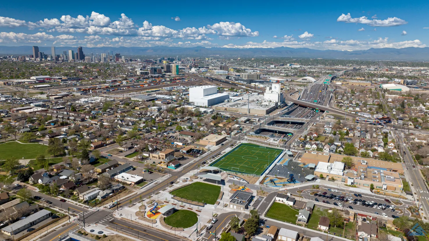
(Source of photo) Hammon, Mary. “Opening of Denver’s New Freeway Cap Park Triggers Gentrification Fears.” 2023. Planetizen.com. 2023. https://www.planetizen.com/news/2023/12/126716-opening-denvers-new-freeway-cap-park-triggers-gentrification-fears.
Reklaitiene, Regina, Regina Grazuleviciene, Audrius Dedele, Dalia Virviciute, Jone Vensloviene, Abdonas Tamosiunas, Migle Baceviciene, et al. 2014. “The Relationship of Green Space, Depressive Symptoms and Perceived General Health in Urban Population.” Scandinavian Journal of Public Health 42 (7): 669–76. https://doi.org/10.1177/1403494814544494.
Rigolon, Alessandro, and Jeremy Németh. 2018. “What Shapes Uneven Access to Urban Amenities? Thick Injustice and the Legacy of Racial Discrimination in Denver’s Parks.” Journal of Planning Education and Research 41 (3): 0739456X1878925. https://doi.org/10.1177/0739456x18789251.
Sachs, David. 2018. “This Shape Explains Denver’s Past, Present and Likely Its Future.” Denverite. December 21, 2018. https://denverite.com/2018/12/21/denver-socioeconomic-map-shape/.
Site Description

The map above is the Redlining Map of Denver and for basic orientation it shows the grid Denver is based on with 2 axes - going north to south is Broadway, and going west to east is Colfax (Nelson and Winling 2023). At the time the redlining maps were made (1935-1940) I-70 and I-25 were yet to be constructed, but where these highways end up going are clearly seen on the redlining map (Nelson and Winling 2023). I-25 runs north to south with a bit of a bend on the southern part; in the redlining map, I-25 would later start in the south east where there were already railroad tracks, then moves northwest to meet with the South Platte River, then moves northward alongside the river. I-70 would later cut through the Globeville, Elyeria, Swansia areas which were the 'hazardous' redlining grade, then went east along an existing road and railroad tracks, and went west along 48th Ave. Those areas that are on the west portion of I-70 were 'hazardous' and 'defiitely declining' redlining grades and the highway cut through pre-existing neighborhoods that were majority immigrant populated (Chen, Chavez-Norgaard, and University of Richmond 2025).
Knowing the orientation of Denver and short context for how and why it is oreinted the way it is, is important for understanding the uneven distribution of urban greenspace and the signifcance behind that. Denver has uneven access to urban greenspace that is rooted in racial discrimination and other injustices from redlining, gerrymandering, segregation, and racially restrictive covenants (Rigolon and Németh 2018). Because parks were a large push of the City Beautiful Movement which was about increasing the city's prestige, the majority of the parks created were in upscale white neighborhoods that paid higher property taxes (Rigolon and Németh 2018). Some of the major or flagship parks in Denver are Cheeseman Park (just north of Colfax and just to the east of Broadway), Washington Park (slender rectangle south of Colfax), and City Park (north of Colfax, east of Broadway). All of those parks are inside the 'inverted L' which can be seen on the redlining map as well as the graphic above. Recently there was research showing that inside the 'inverted L' (east of I-25 and south of I-70) are predominately white, not vulnerable to displacement, more educated, and have more trees (Sachs 2018). Since the series of maps above were made, trees planted by the city are outside of the 'inverted L' (Sachs 2021). While there has been work to undo the inequitable effects redlining policies and create hopefully someday equal access and use to urban greenspace - to this day those flagship parks predominately still serve the city's most affluent groups of whom are White (Cernansky 2019).
For this project, because the focus is on the relationship between a health outcome (% of depression prevalence) and urban greenspace, the idea or theory behind the 'inverted L' will guide further analyses to see first if vegetation related variables and % of depression prevalence have a predictive relationship and second if it does - does it follow the 'inverted L' pattern seen in socioeconomic related variables. I would hypothesize that there would be higher % of depression prevalence outside of the 'inverted L' because there is less greenspace there.
Citations:
Cernansky, Rachel. 2019. “Unequal Access to Parks in Denver Has Roots in History.” Collective Colorado. July 16, 2019. https://collective.coloradotrust.org/stories/unequal-access-to-parks-in-denver-has-roots-in-history/.
Chen, Victor, Stefan Chavez-Norgaard, and University of Richmond. 2025. “Mapping Inequality: Denver.” Mapping Inequality: Redlining in New Deal America. University of Richmond. 2025. https://dsl.richmond.edu/panorama/redlining/map/CO/Denver/context#loc=12/39.6994/-104.9581.
Nelson, Robert K, and LaDale Winling. 2023. “Mapping Inequality: Redlining in New Deal America.” In American Panorama: An Atlas of United States History, edited by Robert K Nelson and Edward L. Ayers. https://dsl.richmond.edu/panorama/redlining.
Rigolon, Alessandro, and Jeremy Németh. 2018. “What Shapes Uneven Access to Urban Amenities? Thick Injustice and the Legacy of Racial Discrimination in Denver’s Parks.” Journal of Planning Education and Research 41 (3): 0739456X1878925. https://doi.org/10.1177/0739456x18789251.
Sachs, David. 2018. “This Shape Explains Denver’s Past, Present and Likely Its Future.” Denverite. December 21, 2018. https://denverite.com/2018/12/21/denver-socioeconomic-map-shape/.
Sachs, David. 2021. “How Denver Is Chipping Away at the Inverted L: Housing and Trees Edition.” Denverite. April 7, 2021. https://denverite.com/2021/04/07/how-denver-is-chipping-away-at-the-inverted-l-housing-and-trees-edition/.
Data Description
* CDC Places Data

CDC Places Data (prior to it being taken down)
CDC Places prior to 2020 was known as 500 Cities, so instead of having full coverage across the US including rural areas, it only included 500 cities (CDC 2021, "About the Places Project"). While in this phase, the datasets also only included chronic diseases (CDC 2021, "About the Places Project"). Since 2020 it has expanded the measures included in the datasets, and these measures included, are increasing each year the datasets are released (CDC 2021, "Measure Definitions"). It appears new sets of data are released every year rather than old/ previous years' datasets being updated (CDC 2021, "About the Places Project").
If curious about the methodology that CDC Places uses and how the data is validated, please visit CDC Places methodology. (Since writing this, this page has been taken down, keeping for purposes of retaining information).
Due this being realted to the Census (which is only done every 10 years) also affects this data in that research will need to be done to see what Census data the year of selected CDC Places data is using (CDC 2021, "About the Places Project"). For example, the 2024 CDC Places data is using the 2020 Census, not the 2010 Census like the prior years of the CDC Places data (CDC 2021, "About the Places Project"). The CDC datasets also differ by geography type or administrative boundaries (CDC 2021, "About the Places Project"). While this project is using Census Tracts as the boundary, there are other options available like U.S. counties, census designated places, and ZIP Code Tabulation Areas (ZCTA's) (CDC 2021, "PLACES"). Depending on the goal of a project, would likely change the geography being used. CDC Places data includes all areas of the United States with 50 or more adult residents (CDC 2021, "About the Places Project").
Prior to the CDC data being taken down, the data was free to access which contributed to Open Data Science efforts. The data was considered public domain and did not require or have a specific license to use or manipulate the data as of 2/2/2025.
(Prior to 2/2/2025) The data itself could be accessed in multiple formats icnluding JSON, GeoJSON (which is what I used), CSV if getting via API. Or, if downloading it can be accessed in even more formats including those listed prior and many others (CDC 2021, "PLACES"). This is worth exploring and considering depending on what project the data is being used for and how the data will be used. As of 2/20/2025 I was able to call the CDC API to get the census tracts associated with the CDC places data without issue; however, once I got to the downloading the health outcome data like asthma, depression, stroke, etc. I wasn't able to access it via the same API call. Instead, I used the Internet Archive to access data that was previously available on the CDC website (CDC 2025, (Internet Archive - CDC Datasets)).
CDC Places Data (via the Internet Archive)
The Internet Archive is a non-profit that has been archiving websites and other digital assests since 1996 (Internet Archive 2009). What they archieve is quite vast including: webpages, books/texts, audio recording, videos (including tv news), images, software, etc. (Internet Archive 2009). They have many different orgnaizations which fund them including the American Library Association and the Biodiversity Heritage Library (Internet Archive 2009). This is free to use and access - their goal is to make knowledge publicly accessible, but there is one exception and it's for books made after 1928 can only be borrowed (Internet Archive 2009). So, this also contributes to Open Science efforts and does not have a particular liecence to access the information the Internet Archive has (Internet Archive 2009)
Anything can be searched in the 'Wayback Machine', their searchbar, looking for a website, book, any of the formats listed previously and it will return many results that will take time to sift through to find what you are looking for (Internet Archive 2014). For this project the focus is the CDC datasets which were taken off the CDC website around January 31st. I was able to access the CDC dataset 2/2/2025 via API call but was unable to call the API after that for the CSV data about health outcomes. This led me to the Internet Archive to access this data that was taken down.
The CDC datasets saved on the Internet Archive are set up differently, and organized by type of CDC dataset, so I navigated to the comma-separated values (csv) because I needed a csv file to merge the depression data with the geometry of the census tracts. There are a ton (2000+) of different CSV datasets available here; there's everything from COVID-19 data, impaired driving deaths, medicaid coverage, the 'Places' data (which is what I needed) and so on (CDC 2025, (Internet Archive - CDC Datasets)). I used the url - "PLACES_Local_Data_for_Better_Health_Census_Tract_Data_2022_release.csv" because I needed the 'Places - local data for better health' for census tracts and chose 2022 because it only had 512M versus 2023 has 617M and 2024 has 726M (CDC 2025, (Internet Archive - CDC Datasets)). Even though I ended up using an API call, the issue was that I knew I would need to download the entire dataset to see what I was working with to set up the API call with the correct spelling/capitalization/etc. I was more comfortable with downloading the 512M than the higher amounts. There was an available metadata csv to download on the Internet Archive as well; however I downloaded it and it didn't tell me the names of columns or anything that would help with the API call (CDC 2025, (Internet Archive - CDC Datasets)). In looking at the downloaded dataset, the data was actually from a mix of years, mainly 2020, but also had some (very few rows) of 2021 and 2022; it also had different capitalization and names for the columns than what the original CDC dataset had. All of this should be kept in mind if you are using the Internet Archive for a dataset but previously had access to the original format. The datasets might be set up differently and while there is data there, it may not be exactly what it was when it was queryed or called through the original source. Despite these complications, I am very grateful that this dataset, as well as all the other CDC datasets are still accessible via the Internet Archive. There are other entities, mostly private or non-profit that have also secured those CDC datasets, so it is possible to find the datasets a different way, but that would likely take more digging and possibly requesting the data instead of anytime access to the Internet Archive.
CDC Places Citations:
CDC Places data accessed previously - https://data.cdc.gov/resource/cwsq-ngmh.geojson (Since writing this, this page has been taken down, keeping for purposes of retaining information).
Center for Disease Control and Prevention (CDC). 2020. “PLACES Methodology.” Centers for Disease Control and Prevention. December 8, 2020. https://www.cdc.gov/places/methodology/index.html. (Since writing this, this page has been taken down, keeping for purposes of retaining information).
Center for Disease Control and Prevention (CDC). 2021. “About the PLACES Project.” Centers for Disease Control and Prevention. October 18, 2021. https://www.cdc.gov/places/about/index.html. (Since writing this, this page has been taken down, keeping for purposes of retaining information).
Centers for Disease Control and Prevention (CDC). 2021. “Measure Definitions.” Centers for Disease Control and Prevention. October 18, 2021. https://www.cdc.gov/places/measure-definitions/index.html. (Since writing this, this page has been taken down, keeping for purposes of retaining information).
Centers for Disease Control and Prevention (CDC). 2021. “PLACES: Local Data for Better Health.” Centers for Disease Control and Prevention. March 8, 2021. https://www.cdc.gov/PLACES. Data initially Accessed via API [2/2/2025] (Since writing this, this page has been taken down, keeping for purposes of retaining information).
Centers for Disease Control and Prevention (CDC). 2024. “Data | Centers for Disease Control and Prevention.” Data.CDC.gov. 2024. https://data.cdc.gov/browse?category=500+Cities+%26+Places&q=2024&sortBy=relevance&tags=places. (Note - this link takes you too all the localties and verstions avialable not the specific one used here). *(Since writing this, this page has been taken down, keeping for purposes of retaining information).
Centers for Disease Control and Prevention (CDC). 2025. “CDC Datasets Uploaded before January 28th, 2025 : Centers for Disease Control and Prevention : Free Download, Borrow, and Streaming : Internet Archive.” Internet Archive - CDC Datasets. January 28, 2025. https://archive.org/details/20250128-cdc-datasets.
Internet Archive. 2009. “About the Internet Archive.” Archive.org. 2009. https://archive.org/about/.
Internet Archive. 2014. “Internet Archive.” Archive.org. 2014. https://archive.org.
* NAIP via Microsoft Planetary Computer STAC API - Multispectral Data


The data source that will be used for the urban green space element of this project is NAIP (National Agricultural Imagery Program) (United States Geological Survey (USGS) - Earth Resources Observation and Science (EROS) Center, n.d.). The NAIP data can be used for many things beyond what this case study aims to do, in fact it is usually used for agriculture and it is worth exploring if it is applicable or useful in other projects, agriculture related and beyond (United States Geological Survey (USGS) - Earth Resources Observation and Science (EROS) Center, n.d.). NAIP is aerial imagery that has a 1m resolution and has coverage for the continental U.S. with either red, blue, green bands, or near infrared, red, green, and blue bands (United States Geological Survey (USGS) -Earth Resources Observation and Science (EROS) Center, n.d.). Similar to satellite imagery, the devices used to capture the images have multiple sensors, each sensor is for a different reflective spectral band in the electromagnetic wavelength (Science Education through Earth Observation for High Schools (SEOS) and European Association of Remote Sensing Laboratories n.d.). A band alone cannot convey much, but the relationship between two or more bands does - these are normalized spectral indices such as NDMI, NDVI, and others (United States Geological Survey (USGS) n.d.). Information on more in detail about remote sensing can be found here (Science Education through Earth Observation for High Schools (SEOS) and European Association of Remote Sensing Laboratories n.d.). NDVI will be used in this project in order to calculate the vegetation statistics. These vegetation statistics will be used to be able to see if those variables can predict % depression prevalence in Denver.
To access the NAIP data the Microsoft Planetary Computer STAC (SpatioTemporal AccessCatalog) API was used. The Microsoft Planetary Copmuter is comprised of 3 main components - the data catalog (this project uses STAC), API's (of which this project will use in order to search for the data needed), and applications (Microsoft. n.d.). The NAIP data is freely accessible via the STAC and a an account is not needed to access this data (the data and API can be used anonymously) (Microsoft. n.d.). In order to interact with the Microsoft Planetary Computer the module 'pystac_client' needs to be imported; it's possible depending on the python environment being used that other imports may be necessary (Microsoft. n.d.). The NAIP data comes from a 'professional' source (USGS) and gathered through aerial imagery that is orthorectified, so there should be a degree of trust in the data, but it depends on how it is being used and what it is being used for (United States Geological Survey (USGS) - Earth Resources Observation and Science (EROS) Center, n.d.).
The NAIP data can vary depending on the timeframe used because the data was collected every 5 years starting in 2003-2009, then was collected at every 3 year interval, and during the year of the collection the imagery is only captured during the agricultural growing season (United States Geological Survey (USGS) - Earth Resources Observation and Science (EROS) Center, n.d.). That is something to keep in mind when setting up the temporal parameter - if 2004 was set as the 'datetime', or December 31, 2003 it wouldn't pull any data - for 2004, that year no imagery was captured, and while 2003 was captured, that day and month wouldn't be within the agricultural growing season (United States Geological Survey (USGS) - Earth Resources Observation and Science (EROS) Center, n.d.). Another element to keep in mind is cloud coverage, of which there will be as much as 10% cloud coverage per tile (United States Geological Survey (USGS) - Earth Resources Observation and Science (EROS) Center, n.d.). When working with imagery is best to get a 'clear' image or images where there is little to no cloud coverage for the best results. Luckily because this data is only captured during the growing season when vegetation is healthiest and would have the greatest percentage reflection and in theory would be less cloud coverage than the non-growing season, which will give in theory better image results anyways due to when the data is taken.
The reason why NAIP was chosen as the data source, was because other sources like 'Harmonized Landsat Sentinel-2', have lower resolution at 30m and that would not be able to capture the structure of the green space, like: edge density, mean patch size, and fragmentation (NASA 2023). The vegetation variables (edge density, mean patch size, and fragmentation) are actually statistics that attempt to quantify the connectivity and structure of green space. Edge density is the total length of all patch areas (perimeter) divded by the total area of the landscape (for this project it's the total area of the census tract) (Ene and Mcgarigal 2023, “(L4) Edge Density”). Mean patch size is the total area of of the patch, and taking the mean of patch size for all patches in the landscape (for this project that will be for all patches in a census tract) (Ene and Mcgarigal 2023, “Landscape Metrics”). Fragmentation is the number of patches or edge density in a specified area (Fahrig 2023). The graphic below helps visualize what some of these terms mean, however it is about habitat so instead, think of the landscape is the census tract and the patch is the vegetation pixel or group of veg pixels in that census tract; the more patches within a census tract, also increases fragmentation and edge density (Fahrig 2023).

NAIP Citations:
Ene, Eduard, and Kevin Mcgarigal. 2023. “Landscape Metrics.” Fragstats.org. 2023. https://fragstats.org/index.php/background/landscape-metrics.
Ene, Eduard, and Kevin Mcgarigal. 2023. “(L4) Edge Density.” Fragstats.org. 2023. https://fragstats.org/index.php/fragstats-metrics/patch-based-metrics/area-and-edge-metrics/l4-edge-density.
Fahrig, Lenore. 2023. “Patch‐Scale Edge Effects Do Not Indicate Landscape‐Scale Fragmentation Effects.” Conservation Letters 17 (1). https://doi.org/10.1111/conl.12992.
GeoNext, and Krishnagopal Halder. 2024. “Getting Started with Microsoft Planetary Computer STAC API.” Medium. March 19, 2024. https://medium.com/@geonextgis/getting-started-with-microsoft-planetary-computer-stac-api-67cbebe96e5e.
Microsoft. n.d. “About the Microsoft Planetary Computer.” Planetarycomputer.microsoft.com. https://planetarycomputer.microsoft.com/docs/overview/about/.
NASA. 2023. “L30 – Harmonized Landsat Sentinel-2: Products Description.” Nasa.gov. 2023. https://hls.gsfc.nasa.gov/products-description/l30/.
Science Education through Earth Observation for High Schools (SEOS), and European Association of Remote Sensing Laboratories. n.d. “Introduction to Remote Sensing.” Seos-Project.eu. Accessed February 22, 2025. https://seos-project.eu/remotesensing/remotesensing-c01-p06.html.
United States Geological Survey (USGS). n.d. “Landsat Surface Reflectance-Derived Spectral Indices | U.S. Geological Survey.” Www.usgs.gov. USGS. Accessed February 22, 2025. https://www.usgs.gov/landsat-missions/landsat-surface-reflectance-derived-spectral-indices.
United States Geological Survey (USGS) - Earth Resources Observation and Science (EROS) Center . 2018. “USGS EROS Archive - Aerial Photography - High Resolution Orthoimagery (HRO) | U.S. Geological Survey.” Www.usgs.gov. July 6, 2018. https://www.usgs.gov/centers/eros/science/usgs-eros-archive-aerial-photography-high-resolution-orthoimagery-hro.
United States Geological Survey (USGS) -Earth Resources Observation and Science (EROS) Center. n.d. “USGS EROS Archive - Aerial Photography - National Agriculture Imagery Program (NAIP) | U.S. Geological Survey.” Www.usgs.gov. https://www.usgs.gov/centers/eros/science/usgs-eros-archive-aerial-photography-national-agriculture-imagery-program-naip.
Methods Description
OLS Regression will be used as the model to find out if there is a statistically significant relationship between depression and greenspace. This will be using the variables of % of depression prevalence and vegeation related variables. Models can be used for different purposes in earth data science, one of which is prediction. Here, the goal is to see if the model can predict the depression prevalence accurately. In order to evaluate the model, calculated error could be looked at or calculate R squared which would say what percent of variation in depression prevalence can be explained by the model. For this project calculated error is chosen.
Important factors when choosing a model is to consider the assumptions about the data and if the model is appropriate given the data. Some important assumptions about OLS regression are: linearity - assuming there is a linear relationship between the two variables, normally distributed error - data shouldn't have long tails, independence - avoid co-linearity of tightly correlated variables, stationarity - parameters of the model should not vary over time, and complete observations - shouldn't have large amounts of no data values.
The data can be manipulated or adjusted to be a better fit. For example:
- No data values can be dropped to account for complete observations using .dropna()
- Log of variables can be taken to make the data more normally distributed and not have long tails using np.log.
- Normalization/standardization of data to account for the different scales of the variables
- Etc.
For this project independence and stationairity are not of major concern, but there are no data values, the data has tails, and the two variables do have very different scales, so the data needs to have the fixes done to fit the model. There is a delicate balance of fitting to overfitting. Potential issues with choosing this model are using the chosen variables, there may not be a linear relationship and so the results may be quite muddy or not relay that there is a relationship between the variables. Another potential issue is overfitting the model - this would mean making so many or enough adjustments to the data to 'fit it' and it results in the model fitting to the noise having very low error and not much can be relayed of a possible relationship between the variables when this happens. Because overfitting in particular is a worry here, a way to avoid that, is cross validation.
Cross validation is when the data is split into a training and a testing set - for this project, the model is trained on 66% of the data and then test the model's performance on the other 33% of the data. This split could be divided differently though like it could be 70% training and 30% testing or something different. This process of spliting the data into training and testing sets can be done iteratively with randomly selected data, but that is with a different type of model than the one used here (random forest model does this iteratively, OLS regression does not).
A way to evaluate the model's results is computing model error. For this project this will be calculated by (% of depression prevalence predicted - measured/actual % of depression prevalence) for all census tracts. This model error will be plotted with a diverging color scheme to see visually what can be noticed and if there any explanation for any bias in the model results.
Personally not having much experience in Earth Data Science and Statistics, I am unfamiliar with other possible models that could be used here. Another one I know of it the Decision Tree Model or Random Forest Model but would need to do more research if other models would be more appropriate here.
Set Up Analysis and Site Plot
# Set Up Analysis Part 1 of 2

# Import libraries to help with ...

# Reproducible file paths
import os # Reproducible file paths
from glob import glob # Find files by pattern
import pathlib # Find the home folder
import time # formatting time
import warnings # Filter warning messages
import zipfile # Work with zip files
from io import BytesIO # Stream binary (zip) files

# Find files by pattern
import numpy as np # adjust images
import matplotlib.pyplot as plt # Overlay pandas and xarry plots, Overlay raster and vector data
import requests # Request data over HTTP

# Work with tabular, vector, and raster data
import cartopy.crs as ccrs # CRSs (Coordinate Reference Systems)
import geopandas as gpd # work with vector data
import geoviews as gv # holoviews extension for data visualization
import hvplot.pandas # Interactive tabular and vector data
import hvplot.xarray # Interactive raster
import pandas as pd # Group and aggregate
import pystac_client # Modify returns from API
import shapely # Perform geometric operations on spatial data
import xarray as xr # Adjust images
import rioxarray as rxr # Work with geospatial raster data
from rioxarray.merge import merge_arrays # Merge rasters

# Processing and regression related
from scipy.ndimage import convolve # Image and signal processing
from sklearn.model_selection import KFold # Cross validation
from scipy.ndimage import label # Labels connected features in an array
from sklearn.linear_model import LinearRegression # Work with linear regression models
from sklearn.model_selection import train_test_split # Split data into subsets - evaluate model
from tqdm.notebook import tqdm # Visualize progress of iterative operations

# import to be able to save plots
import holoviews as hv # be able to save hvplots

# Suppress third party warnings - 'ignore'
warnings.simplefilter('ignore')

# Prevent GDAL from quitting due to momentary disruptions
os.environ["GDAL_HTTP_MAX_RETRY"] = "5"
os.environ["GDAL_HTTP_RETRY_DELAY"] = "1"
# Set Up Analysis Part 2 of 2

# Set up census tract path
# Define and create the project data directory
den_census_tracts_data_dir = os.path.join(
    pathlib.Path.home(),
    'documents',
    'earth-analytics',
    'urban_greenspace_denver'
)
os.makedirs(den_census_tracts_data_dir, exist_ok=True)

# Call the data dir to confirm location
den_census_tracts_data_dir
'/Users/briannagleason/documents/earth-analytics/urban_greenspace_denver'
# Download the census tracts from CDC (only once) Part 1 of 1

# Define info for census tract download
den_census_tracts_dir = os.path.join(den_census_tracts_data_dir, 'denver-tract')
os.makedirs(den_census_tracts_dir, exist_ok=True)
den_census_tracts_path = os.path.join(den_census_tracts_dir, '*.shp')

# Only download once (conditional statement)
if not os.path.exists(den_census_tracts_path):
    den_census_tracts_url = (
    'https://data.cdc.gov/download/x7zy-2xmx/application%2Fzip'
    )
    den_census_tracts_gdf = gpd.read_file(den_census_tracts_url)
    denver_tracts_gdf = den_census_tracts_gdf[den_census_tracts_gdf.PlaceName=='Denver']
    denver_tracts_gdf.to_file(den_census_tracts_path, index=False)

# Load in the census tract data
denver_tracts_gdf = gpd.read_file(den_census_tracts_path)

# Call the chicago tracts gdf to see it
denver_tracts_gdf.head()
| place2010 | tract2010 | ST | PlaceName | plctract10 | PlcTrPop10 | geometry | |
|---|---|---|---|---|---|---|---|
| 0 | 0820000 | 08031000102 | 08 | Denver | 0820000-08031000102 | 3109 | POLYGON ((-11691351.798 4834636.885, -11691351... |
| 1 | 0820000 | 08031000201 | 08 | Denver | 0820000-08031000201 | 3874 | POLYGON ((-11688301.532 4835632.272, -11688302... |
| 2 | 0820000 | 08031000202 | 08 | Denver | 0820000-08031000202 | 3916 | POLYGON ((-11688362.201 4834372.228, -11688360... |
| 3 | 0820000 | 08031000301 | 08 | Denver | 0820000-08031000301 | 5003 | POLYGON ((-11691355.36 4833538.467, -11691357.... |
| 4 | 0820000 | 08031000302 | 08 | Denver | 0820000-08031000302 | 4036 | POLYGON ((-11692926.635 4832494.047, -11692925... |
# Download the census tracts for state of CO (only once) Part 1 of 1

# Define info for census tract download
den_tiger_tracts_dir = os.path.join(den_census_tracts_data_dir, 'colorado-tracts')
os.makedirs(den_tiger_tracts_dir, exist_ok=True)
den_tiger_tracts_path = os.path.join(den_tiger_tracts_dir, '*.shp')

# Only download once (conditional statement)
if not os.path.exists(den_tiger_tracts_path):
    co_tiger_tracts_url = (
    'https://www2.census.gov/geo/tiger/TIGER2024/TRACT/tl_2024_08_tract.zip'
    )
    co_tiger_tracts_gdf = gpd.read_file(co_tiger_tracts_url)
    # COUNTYFP 031 is Denver County which in this case is also the City of Denver
    # It's a City and a County
    den_tiger_tracts_gdf = co_tiger_tracts_gdf[co_tiger_tracts_gdf.COUNTYFP=='031']
    den_tiger_tracts_gdf.to_file(den_tiger_tracts_path, index=False)

# Load in the census tract data
den_tiger_tracts_gdf = gpd.read_file(den_tiger_tracts_path)

# Call the chicago tracts gdf to see it
den_tiger_tracts_gdf.head()
| STATEFP | COUNTYFP | TRACTCE | GEOID | GEOIDFQ | NAME | NAMELSAD | MTFCC | FUNCSTAT | ALAND | AWATER | INTPTLAT | INTPTLON | geometry | |
|---|---|---|---|---|---|---|---|---|---|---|---|---|---|---|
| 0 | 08 | 031 | 004404 | 08031004404 | 1400000US08031004404 | 44.04 | Census Tract 44.04 | G5020 | S | 1304208 | 0 | +39.7365094 | -104.8940558 | POLYGON ((-104.90346 39.73899, -104.90346 39.7... |
| 1 | 08 | 031 | 004403 | 08031004403 | 1400000US08031004403 | 44.03 | Census Tract 44.03 | G5020 | S | 1465389 | 0 | +39.7443925 | -104.8948130 | POLYGON ((-104.90346 39.74561, -104.90346 39.7... |
| 2 | 08 | 031 | 003701 | 08031003701 | 1400000US08031003701 | 37.01 | Census Tract 37.01 | G5020 | S | 1873267 | 120383 | +39.7444161 | -104.9509827 | POLYGON ((-104.95979 39.7452, -104.95978 39.74... |
| 3 | 08 | 031 | 003702 | 08031003702 | 1400000US08031003702 | 37.02 | Census Tract 37.02 | G5020 | S | 706200 | 0 | +39.7365218 | -104.9543646 | POLYGON ((-104.95979 39.73504, -104.95979 39.7... |
| 4 | 08 | 031 | 003703 | 08031003703 | 1400000US08031003703 | 37.03 | Census Tract 37.03 | G5020 | S | 681502 | 0 | +39.7361181 | -104.9450408 | POLYGON ((-104.94949 39.73242, -104.94949 39.7... |
# Perform a spatial join for census tracts at least partially
# within City of Denver boundary

# this new gdf needs to be joined to the previous one from CDC which
# is already clipped to the city boundary, so no need to download a
# seperate city boundary shapefile which reduces the amount of things
# being downloaded

# Define new variable for the joind gdf
joined_den_tracts_gdf = (
    gpd.sjoin(
        # TIGER tracts gdf - only need tracts that intersect with..
        den_tiger_tracts_gdf.to_crs(ccrs.Mercator()),
        # CDC tracts gdf - which are already clipped to the Chicago city boundary
        denver_tracts_gdf.to_crs(ccrs.Mercator()),
        # Specify type of join ("inner", "left", "right")
        how="inner",
        # Specify the spatial relationship ("intersects", "within", "contains")
        predicate="intersects"
        )
)

# Explore the result
joined_den_tracts_gdf.head()
| STATEFP | COUNTYFP | TRACTCE | GEOID | GEOIDFQ | NAME | NAMELSAD | MTFCC | FUNCSTAT | ALAND | ... | INTPTLAT | INTPTLON | geometry | index_right | place2010 | tract2010 | ST | PlaceName | plctract10 | PlcTrPop10 | |
|---|---|---|---|---|---|---|---|---|---|---|---|---|---|---|---|---|---|---|---|---|---|
| 0 | 08 | 031 | 004404 | 08031004404 | 1400000US08031004404 | 44.04 | Census Tract 44.04 | G5020 | S | 1304208 | ... | +39.7365094 | -104.8940558 | POLYGON ((-11677799.972 4800763.868, -11677799... | 90 | 0820000 | 08031004405 | 08 | Denver | 0820000-08031004405 | 7316 |
| 0 | 08 | 031 | 004404 | 08031004404 | 1400000US08031004404 | 44.04 | Census Tract 44.04 | G5020 | S | 1304208 | ... | +39.7365094 | -104.8940558 | POLYGON ((-11677799.972 4800763.868, -11677799... | 89 | 0820000 | 08031004404 | 08 | Denver | 0820000-08031004404 | 5978 |
| 1 | 08 | 031 | 004403 | 08031004403 | 1400000US08031004403 | 44.03 | Census Tract 44.03 | G5020 | S | 1465389 | ... | +39.7443925 | -104.8948130 | POLYGON ((-11677800.084 4801719.178, -11677799... | 89 | 0820000 | 08031004404 | 08 | Denver | 0820000-08031004404 | 5978 |
| 1 | 08 | 031 | 004403 | 08031004403 | 1400000US08031004403 | 44.03 | Census Tract 44.03 | G5020 | S | 1465389 | ... | +39.7443925 | -104.8948130 | POLYGON ((-11677800.084 4801719.178, -11677799... | 88 | 0820000 | 08031004403 | 08 | Denver | 0820000-08031004403 | 4213 |
| 1 | 08 | 031 | 004403 | 08031004403 | 1400000US08031004403 | 44.03 | Census Tract 44.03 | G5020 | S | 1465389 | ... | +39.7443925 | -104.8948130 | POLYGON ((-11677800.084 4801719.178, -11677799... | 80 | 0820000 | 08031004107 | 08 | Denver | 0820000-08031004107 | 3810 |
5 rows × 21 columns
# Try to see how many rows there are because I think there's duplicates
num_rows = joined_den_tracts_gdf.shape[0]
print("Number of rows:", num_rows)
Number of rows: 637
# Drop duplicate geometries

# Normalize the geometry column to ensure consistent representation
joined_den_tracts_gdf['geometry'] = joined_den_tracts_gdf.geometry.normalize()

# Drop duplicate rows based on the geometry column
dropped_joined_den_tracts_gdf = joined_den_tracts_gdf.drop_duplicates(subset='geometry')

# Call the gdf to see it
dropped_joined_den_tracts_gdf.head()
| STATEFP | COUNTYFP | TRACTCE | GEOID | GEOIDFQ | NAME | NAMELSAD | MTFCC | FUNCSTAT | ALAND | ... | INTPTLAT | INTPTLON | geometry | index_right | place2010 | tract2010 | ST | PlaceName | plctract10 | PlcTrPop10 | |
|---|---|---|---|---|---|---|---|---|---|---|---|---|---|---|---|---|---|---|---|---|---|
| 0 | 08 | 031 | 004404 | 08031004404 | 1400000US08031004404 | 44.04 | Census Tract 44.04 | G5020 | S | 1304208 | ... | +39.7365094 | -104.8940558 | POLYGON ((-11677800.195 4800722.197, -11677799... | 90 | 0820000 | 08031004405 | 08 | Denver | 0820000-08031004405 | 7316 |
| 1 | 08 | 031 | 004403 | 08031004403 | 1400000US08031004403 | 44.03 | Census Tract 44.03 | G5020 | S | 1465389 | ... | +39.7443925 | -104.8948130 | POLYGON ((-11677800.084 4801719.178, -11677799... | 89 | 0820000 | 08031004404 | 08 | Denver | 0820000-08031004404 | 5978 |
| 2 | 08 | 031 | 003701 | 08031003701 | 1400000US08031003701 | 37.01 | Census Tract 37.01 | G5020 | S | 1873267 | ... | +39.7444161 | -104.9509827 | POLYGON ((-11684070.377 4801596.893, -11684070... | 83 | 0820000 | 08031004301 | 08 | Denver | 0820000-08031004301 | 4469 |
| 3 | 08 | 031 | 003702 | 08031003702 | 1400000US08031003702 | 37.02 | Census Tract 37.02 | G5020 | S | 706200 | ... | +39.7365218 | -104.9543646 | POLYGON ((-11684070.933 4799965.66, -11684070.... | 57 | 0820000 | 08031003300 | 08 | Denver | 0820000-08031003300 | 3099 |
| 4 | 08 | 031 | 003703 | 08031003703 | 1400000US08031003703 | 37.03 | Census Tract 37.03 | G5020 | S | 681502 | ... | +39.7361181 | -104.9450408 | POLYGON ((-11682924.12 4799771.02, -11682924.0... | 57 | 0820000 | 08031003300 | 08 | Denver | 0820000-08031003300 | 3099 |
5 rows × 21 columns
# Site plot -- Census tracts with satellite imagery in the background

# Create new variable for plot in order to save it later
joined_denver_tracts_plot = dropped_joined_den_tracts_gdf.to_crs(
# Use hvplot to plot and set parameters
ccrs.Mercator()).hvplot(
    geo=True, crs=ccrs.Mercator(),
    tiles='EsriImagery',
    title='City and County of Denver - Site Plot of Census Tracts',
    fill_color=None, line_color='darkorange',
    line_width=3, #frame_width=600
    width=700 , height=500
)

# Save the plot as html to be able to display online
hv.save(joined_denver_tracts_plot, 'joined_den_site_plot_using_tiger_and_cdc.html')

# Display the plot
joined_denver_tracts_plot
The City and County of Denver census tracts show how the northeast has much larger area of tracts than the rest of the city. The largest one is the airport in the largest tract in the northeast corner. It may be worth considering taking out the airport census tract if there isn't housing, but becuase this is an initial look and project with Denver data I want to see how it plays out as is. Due to the airport tract the city ranges roughly 1 degree latitude and longitude. Visually the greenspace in the city appears mostly in the 'inverted L' as well as in the southwest corner where there is a small lake (Marston Lake). As mentioned in the site description the 'inverted L' tracing roughly I-25 going north to south and I-70 going west to east (Sachs 2018). Those highways are highly visible even in with the census tracts overlay - the highways look grey with highly developed areas around them. The 'inverted L' will continue to play a role in analysis of plots and data.
Location of greenspace is also tied to the effects of redlining as mentioned in the site description (Chen, Chavez-Norgaard, and University of Richmond 2025). So there may be possible connections between socio-economic data, depression prevalence, and urban greenspace. Which leaves room for further study.
Citations:
Chen, Victor, Stefan Chavez-Norgaard, and University of Richmond. 2025. “Mapping Inequality: Denver.” Mapping Inequality: Redlining in New Deal America. University of Richmond. 2025. https://dsl.richmond.edu/panorama/redlining/map/CO/Denver/context#loc=12/39.6994/-104.9581.
Sachs, David. 2018. “This Shape Explains Denver’s Past, Present and Likely Its Future.” Denverite. December 21, 2018. https://denverite.com/2018/12/21/denver-socioeconomic-map-shape/.
Depression Data Wrangle
Links to asthma data - for reference (both original and archived)
"https://data.cdc.gov/api/views/cwsq-ngmh/rows.csv?accessType=DOWNLOAD"
# Set up a path for the depression data
den_cdc_depression_path = os.path.join(den_census_tracts_data_dir, 'asthma.csv')

# Download depression data (only once)
if not os.path.exists(den_cdc_depression_path):
    # Define new variable for url
    cdc_places_tracts_url = (

        "https://archive.org/download/20250128-cdc-datasets/PLACES_Local_Data_for_Better_Health_Census_Tract_Data_2022_release.csv"
        #"&StateAbbr=CO"
        #"&CountyName=Denver"
        #"&Measureid=DEPRESSION"
        #"&$limit=1500"
    )

    # Make a request to the URL and show progress with tqdm
    print("Downloading data...")
    response = requests.get(cdc_places_tracts_url, stream=True)

    # Check for successful request (status code 200)
    if response.status_code == 200:
        # Total size of the response in bytes for tqdm
        total_size = int(response.headers.get('content-length', 0))

        # Download and save the file in chunks, updating the progress bar
        with open(den_cdc_depression_path, 'wb') as f, tqdm(
            total=total_size, unit='B', unit_scale=True, desc="Downloading depression data"
        ) as pbar:
            for data in response.iter_content(chunk_size=1024):
                f.write(data)
                pbar.update(len(data))  # Update the progress bar with the chunk size
    else:
        print(f"Failed to download data. HTTP Status code: {response.status_code}")

    # After download, process the CSV and load into a DataFrame
    print("Processing the downloaded data...")

    # Define new variable for dataframe
    cdc_df = (
        # Read a CSV file into a dataframe
        pd.read_csv(den_cdc_depression_path)
        # Replace column names as needed - 'old_name':'new_name'
        .rename(columns={
            'Data_Value': 'depression',
            'Low_Confidence_Limit': 'depression_ci_low',
            'High_Confidence_Limit': 'depression_ci_high',
            'LocationName': 'tract'})
        # Select specifc columns needed/wanted with double brackets
        [[
            'MeasureId',
            'CountyName',
            'Year',
            'tract',
            'depression', 'depression_ci_low', 'depression_ci_high', 'Data_Value_Unit',
            'TotalPopulation'
        ]]
    )

    # Filter based on multiple conditions:
    den_cdc_depression_df = cdc_df[
        # Select the health outcome wanted from the measure id
        (cdc_df['MeasureId'] =='DEPRESSION') &
        # Select the county name
        (cdc_df['CountyName'] =='Denver')
        # If the county name occurs in more than one state,
        # the sateabbr would need to be chosen and included in this
        # selection and in the columns wanted above
    ]

    # Save dataframe to a CSV (tabular data) file
    den_cdc_depression_df.to_csv(
        den_cdc_depression_path,
        # Prevent a new index column from being created
        index=False
        )

# Load in depression data
den_cdc_depression_df = pd.read_csv(den_cdc_depression_path)

# Preview depression data
den_cdc_depression_df
| MeasureId | CountyName | Year | tract | depression | depression_ci_low | depression_ci_high | Data_Value_Unit | TotalPopulation | |
|---|---|---|---|---|---|---|---|---|---|
| 0 | DEPRESSION | Denver | 2020 | 8031001301 | 20.5 | 19.6 | 21.5 | % | 4972 |
| 1 | DEPRESSION | Denver | 2020 | 8031000600 | 19.5 | 18.4 | 20.9 | % | 2552 |
| 2 | DEPRESSION | Denver | 2020 | 8031001402 | 20.3 | 19.5 | 21.0 | % | 4070 |
| 3 | DEPRESSION | Denver | 2020 | 8031001800 | 22.9 | 21.3 | 24.7 | % | 3209 |
| 4 | DEPRESSION | Denver | 2020 | 8031000301 | 20.0 | 19.1 | 21.0 | % | 5003 |
| ... | ... | ... | ... | ... | ... | ... | ... | ... | ... |
| 138 | DEPRESSION | Denver | 2020 | 8031002802 | 21.5 | 20.6 | 22.5 | % | 4213 |
| 139 | DEPRESSION | Denver | 2020 | 8031003202 | 19.6 | 18.7 | 20.6 | % | 3001 |
| 140 | DEPRESSION | Denver | 2020 | 8031002901 | 21.2 | 19.9 | 22.7 | % | 2602 |
| 141 | DEPRESSION | Denver | 2020 | 8031008391 | 20.0 | 19.2 | 20.8 | % | 7020 |
| 142 | DEPRESSION | Denver | 2020 | 8031004202 | 20.2 | 19.3 | 21.1 | % | 4109 |
143 rows × 9 columns
# Change tract identifier datatype for merging
dropped_joined_den_tracts_gdf.tract2010 = dropped_joined_den_tracts_gdf.tract2010.astype('int64')

# Merge census data with geometry
den_tract_cdc_gdf = (
    # Census tracts gdf
    dropped_joined_den_tracts_gdf
    # Use the .merge() method
    .merge(
        # Depression prevalence dataframe
        den_cdc_depression_df,
        # Specify the column/index to merge on for Census tracts gdf
        left_on='tract2010',
        # Specify the column/index to merge on for the depression dataframe
        right_on='tract',
        # Specify type of join ("inner", "left", "right")
        how='inner'
        )
)

# Plot depression data as chloropleth
den_chloropleth_depression_by_tract = (
# Use EsriImagery tiles for the background
(   gv.tile_sources.EsriImagery
    *
    gv.Polygons(
        # Change gdf CRS to mercator
        den_tract_cdc_gdf.to_crs(ccrs.Mercator()),
        # Set variables for the plot
        vdims=['depression', 'tract2010'],
        # Set CRS to Mercator
        crs=ccrs.Mercator()
    ).opts(
        # Add a colorbar and label
        color='depression', colorbar=True,
        clabel='% of Depression Prevalence in Popultation',
        tools=['hover'])
).opts(
    # Plot size, title, and axes labels
    title= 'Denver - Depression Prevalence by Census Tract',
    # Set the width and the height
    width=800, height=500,
    # Drop the axes labels
    xaxis=None, yaxis=None,
    )
)

# Save the plot as html to be able to display online
hv.save(den_chloropleth_depression_by_tract, 'den_chloropleth_depression_by_tract.html')

# Display the plot
den_chloropleth_depression_by_tract
# Call the denver cdc gdf to see it
den_tract_cdc_gdf.head()
| STATEFP | COUNTYFP | TRACTCE | GEOID | GEOIDFQ | NAME | NAMELSAD | MTFCC | FUNCSTAT | ALAND | ... | PlcTrPop10 | MeasureId | CountyName | Year | tract | depression | depression_ci_low | depression_ci_high | Data_Value_Unit | TotalPopulation | |
|---|---|---|---|---|---|---|---|---|---|---|---|---|---|---|---|---|---|---|---|---|---|
| 0 | 08 | 031 | 004404 | 08031004404 | 1400000US08031004404 | 44.04 | Census Tract 44.04 | G5020 | S | 1304208 | ... | 7316 | DEPRESSION | Denver | 2020 | 8031004405 | 20.7 | 19.6 | 22.0 | % | 7316 |
| 1 | 08 | 031 | 004403 | 08031004403 | 1400000US08031004403 | 44.03 | Census Tract 44.03 | G5020 | S | 1465389 | ... | 5978 | DEPRESSION | Denver | 2020 | 8031004404 | 21.6 | 20.7 | 22.6 | % | 5978 |
| 2 | 08 | 031 | 003701 | 08031003701 | 1400000US08031003701 | 37.01 | Census Tract 37.01 | G5020 | S | 1873267 | ... | 4469 | DEPRESSION | Denver | 2020 | 8031004301 | 20.5 | 19.4 | 21.6 | % | 4469 |
| 3 | 08 | 031 | 003702 | 08031003702 | 1400000US08031003702 | 37.02 | Census Tract 37.02 | G5020 | S | 706200 | ... | 3099 | DEPRESSION | Denver | 2020 | 8031003300 | 20.4 | 19.4 | 21.6 | % | 3099 |
| 4 | 08 | 031 | 003703 | 08031003703 | 1400000US08031003703 | 37.03 | Census Tract 37.03 | G5020 | S | 681502 | ... | 3099 | DEPRESSION | Denver | 2020 | 8031003300 | 20.4 | 19.4 | 21.6 | % | 3099 |
5 rows × 30 columns
Visually, it appears that the west side is slightly darker shades of blue than the west half of the city - so higher % prevalence of depression, with one census tract in particular that appears to be an outlier tract in the northwest. This one census tract has the highest % prevalence of depression which is interesting and will be kept in mind for future analysis. The lighter shades of blue, lower % prevalence of depression are located mostly in the central east and central south east, with a few larger size census tracts in the central north that are also lower % prevalence.
This somewhat line up with the idea of the 'inverted L' having the lower % prevalence of depression in the central west and southwest, but that's not 100% true given some of the tracts beyond the 'inverted L' do have lower % prevalence rates as well (Sachs 2018). There are clear connections in the research made between greenspace and depression, so it will be interesting to see if there is a relationship between urban greenspace and % depression prevalence in further analyses (Reklaitiene et al. 2014). Additionally, the 'inverted L' will continue to be looked at or kept in mind in further analyses (Sachs 2018).
Citations:
Reklaitiene, Regina, Regina Grazuleviciene, Audrius Dedele, Dalia Virviciute, Jone Vensloviene, Abdonas Tamosiunas, Migle Baceviciene, et al. 2014. “The Relationship of Green Space, Depressive Symptoms and Perceived General Health in Urban Population.” Scandinavian Journal of Public Health 42 (7): 669–76. https://doi.org/10.1177/1403494814544494.
Sachs, David. 2018. “This Shape Explains Denver’s Past, Present and Likely Its Future.” Denverite. December 21, 2018. https://denverite.com/2018/12/21/denver-socioeconomic-map-shape/.
NAIP Wrangle
# Connect to the planetary computer catalog
e84_catalog = pystac_client.Client.open(
    "https://planetarycomputer.microsoft.com/api/stac/v1"
)
e84_catalog.title
'Microsoft Planetary Computer STAC API'
Get Data URLs
# Convert geometry to lat/lon for STAC
den_tract_latlon_gdf = den_tract_cdc_gdf.to_crs(4326)

# Define a path to save NDVI stats
den_ndvi_stats_path = os.path.join(den_census_tracts_data_dir, 'denver-ndvi-stats.csv')

# Check for existing data - do not access duplicate tracts

# Create a list to accumulate downloaded tracts
den_downloaded_tracts = []
# If Else statement to control specifc blocks of code
# Code to execute if the condition is true
if os.path.exists(den_ndvi_stats_path):
    den_ndvi_stats_df = pd.read_csv(den_ndvi_stats_path)
    den_downloaded_tracts = den_ndvi_stats_df.tract.values
# Code to execute if the condition is false
else:
    print('No census tracts downloaded so far')


# Loop through each census tract

# Create list of dataframes, list needs to be outside of loop
den_scene_dfs = []
# Start for loop
for i, den_tract_values in tqdm(den_tract_latlon_gdf.iterrows(), ncols=100):
    den_tract = den_tract_values.tract
    # Check if statistics are already downloaded for this tract
    if not (den_tract in den_downloaded_tracts):
        # Retry up to 5 times in case of a momentary disruption
        i = 0
        retry_limit = 5
        # Loop for executing code block as long as specified condition is true
        while i < retry_limit:
            # Try accessing the STAC
            try:
                # Search for tiles
                naip_search = e84_catalog.search(
                    # In the NAIP collection
                    collections=["naip"],
                    # That intersect with geometry of census tracts
                    intersects=shapely.to_geojson(den_tract_values.geometry),
                    # In the year 2021
                    datetime="2021"
                )

                # Build dataframe with tracts and tile urls
                den_scene_dfs.append(pd.DataFrame(dict(
                    tract=den_tract,
                    # Convert datetime value to a pandas Timestamp, then extract just the date
                    date=[pd.to_datetime(scene.datetime).date()
                          # of the items in the NAIP search
                          for scene in naip_search.items()],
                    # Reference image from the assets folder of the items in the NAIP search?
                    rgbir_href=[scene.assets['image'].href for scene in naip_search.items()],
                )))
                # Add break to prevent long waits during debugging
                break
            # Try again in case of an APIError
            except pystac_client.exceptions.APIError:
                print(
                    f'Could not connect with STAC server. '
                    f'Retrying tract {den_tract}...')
                time.sleep(2)
                i += 1
                # Skip the rest of the current iteration and move on to the next one
                continue

# Concatenate the url dataframes
# Code to execute if the condition is true
if den_scene_dfs:
    den_scene_df = pd.concat(den_scene_dfs).reset_index(drop=True)
# Code to execute if the condition is false
else:
    den_scene_df = None

# Preview the URL DataFrame
den_scene_df.head()
No census tracts downloaded so far
0it [00:00, ?it/s]
| tract | date | rgbir_href | |
|---|---|---|---|
| 0 | 8031004405 | 2021-07-28 | https://naipeuwest.blob.core.windows.net/naip/... |
| 1 | 8031004404 | 2021-07-28 | https://naipeuwest.blob.core.windows.net/naip/... |
| 2 | 8031004404 | 2021-07-28 | https://naipeuwest.blob.core.windows.net/naip/... |
| 3 | 8031004301 | 2021-07-28 | https://naipeuwest.blob.core.windows.net/naip/... |
| 4 | 8031004301 | 2021-07-28 | https://naipeuwest.blob.core.windows.net/naip/... |
# See dropped_joined_den_tracts because the merge
# below didn't work because of an index error
dropped_joined_den_tracts_gdf.head()
| STATEFP | COUNTYFP | TRACTCE | GEOID | GEOIDFQ | NAME | NAMELSAD | MTFCC | FUNCSTAT | ALAND | ... | INTPTLAT | INTPTLON | geometry | index_right | place2010 | tract2010 | ST | PlaceName | plctract10 | PlcTrPop10 | |
|---|---|---|---|---|---|---|---|---|---|---|---|---|---|---|---|---|---|---|---|---|---|
| 0 | 08 | 031 | 004404 | 08031004404 | 1400000US08031004404 | 44.04 | Census Tract 44.04 | G5020 | S | 1304208 | ... | +39.7365094 | -104.8940558 | POLYGON ((-11677800.195 4800722.197, -11677799... | 90 | 0820000 | 8031004405 | 08 | Denver | 0820000-08031004405 | 7316 |
| 1 | 08 | 031 | 004403 | 08031004403 | 1400000US08031004403 | 44.03 | Census Tract 44.03 | G5020 | S | 1465389 | ... | +39.7443925 | -104.8948130 | POLYGON ((-11677800.084 4801719.178, -11677799... | 89 | 0820000 | 8031004404 | 08 | Denver | 0820000-08031004404 | 5978 |
| 2 | 08 | 031 | 003701 | 08031003701 | 1400000US08031003701 | 37.01 | Census Tract 37.01 | G5020 | S | 1873267 | ... | +39.7444161 | -104.9509827 | POLYGON ((-11684070.377 4801596.893, -11684070... | 83 | 0820000 | 8031004301 | 08 | Denver | 0820000-08031004301 | 4469 |
| 3 | 08 | 031 | 003702 | 08031003702 | 1400000US08031003702 | 37.02 | Census Tract 37.02 | G5020 | S | 706200 | ... | +39.7365218 | -104.9543646 | POLYGON ((-11684070.933 4799965.66, -11684070.... | 57 | 0820000 | 8031003300 | 08 | Denver | 0820000-08031003300 | 3099 |
| 4 | 08 | 031 | 003703 | 08031003703 | 1400000US08031003703 | 37.03 | Census Tract 37.03 | G5020 | S | 681502 | ... | +39.7361181 | -104.9450408 | POLYGON ((-11682924.12 4799771.02, -11682924.0... | 57 | 0820000 | 8031003300 | 08 | Denver | 0820000-08031003300 | 3099 |
5 rows × 21 columns
""" Uncomment the double comments (##) for code if the merge doesn't
 work below - after I ran it once, it wouldn't let me go back and
 re run it """

# dropped_joined_den_tracts_gdf has a '0' in front of all
# the values for tract2010 (because the stateFP is 08). But...
# the NAIP automatically dropped the '0' in front of all the
# values for the 'tract' column.

# Create a copy of dropped_joined_den_tracts_gdf to perserve the original
## stripped_den_census_tracts_gdf = dropped_joined_den_tracts_gdf.copy()

# Remove/strip the leading '0' from the values of the 'tract2010'
# column of the gdf in order to index correctly
## stripped_den_census_tracts_gdf['tract2010'
    ##] = stripped_den_census_tracts_gdf['tract2010'].str.lstrip('0')

# Call the gdf to make sure that worked
##stripped_den_census_tracts_gdf
" Uncomment the double comments (##) for code if the merge doesn't \n work below - after I ran it once, it wouldn't let me go back and \n re run it "
Compute NDVI Stats
# Create conditional statement
if not den_scene_df is None:
    # Create empty list outside of for loop to save results back to
    all_den_ndvi_dfs = []
    # Loop through the census tracts with URLs
    for tract, tract_date_gdf in tqdm(den_scene_df.groupby('tract')):
        # Open all images for tract
        all_den_tile_das = []
        # Create for loop, iterate over rows
        for _, href_s in tract_date_gdf.iterrows():
            # Open vsi connection to data
            all_den_tile_da = rxr.open_rasterio(
                # File path/url to the multispectral image
                href_s.rgbir_href,
                # Create masked array, then remove any single-dimensional axes from it
                masked=True).squeeze()

            # Crop data to the bounding box of the census tract
            # Create the boundary
            all_den_boundary = (
                # Using the census tract gdf
                den_tract_cdc_gdf
                # Set the 'tract2010' as the index of the gdf
                .set_index('tract2010')
                # Select the tracts from the gdf
                .loc[[tract]]
                # Set to the same CRS as the images for the tracts
                .to_crs(all_den_tile_da.rio.crs)
                # Access the geometry of the tracts to perform further operations
                .geometry
            )
            # Crop the data to bounding box
            all_den_crop_da = all_den_tile_da.rio.clip_box(
                # Compute bounding box (min and max coordinates) of census tract geometry
                *all_den_boundary.envelope.total_bounds,
                # Expand bounding box slightly beyond its original extent to ensure full coverage
                auto_expand=True)

            # Clip data to the boundary of the census tract
            all_den_clip_da = all_den_crop_da.rio.clip(all_den_boundary, all_touched=True)

            # Compute NDVI ((NIR - Red)/(NIR + Red))
            all_den_ndvi_da = (
                (all_den_clip_da.sel(band=4) - all_den_clip_da.sel(band=1))
                / (all_den_clip_da.sel(band=4) + all_den_clip_da.sel(band=1))
            )

            # Accumulate result
            all_den_tile_das.append(all_den_ndvi_da)

        # Merge data
        all_den_scene_da = merge_arrays(all_den_tile_das)

        # Mask vegetation
        all_den_veg_mask = (all_den_scene_da>.3)

        # Calculate statistics and save data to file
        # Calculate total number of non-missing (valid) pixels in the merged raster
        total_pixels = all_den_scene_da.notnull().sum()
        # Calculates total number of pixels that are classified as vegetation
        veg_pixels = all_den_veg_mask.sum()

        # Calculate mean patch size
        # Label the connected areas
        all_labeled_patches, all_num_patches = label(all_den_veg_mask)
        # Count patch pixels, ignoring background at patch 0
        all_patch_sizes = np.bincount(all_labeled_patches.ravel())[1:]
        # Get the mean
        all_mean_patch_size = all_patch_sizes.mean()

        # Calculate edge density
        all_kernel = np.array([
            [1, 1, 1],
            [1, -8, 1],
            [1, 1, 1]])

        # Apply convolution to the vegetation mask
        all_den_edges = convolve(
            # Input array - the array to apply convolution on
            all_den_veg_mask,
            # Kernel array - the smaller array that defines the filter to be applied
            all_kernel,
            # Input array is extended beyond its boundaries by -
            # filling all values beyond the edge with the same constant value
            mode='constant')

        # Calculate edge density =
        # count of edge pixels present / total number of pixels in the veg_mask
        all_den_edge_density = np.sum(all_den_edges != 0) / all_den_veg_mask.size

        # Add a row to the statistics file for this tract
        pd.DataFrame(dict(
            # Unique identifier for a given tract
            tract=[tract],
            # Cast total number of pixels to an integer
            total_pixels=[int(total_pixels)],
            # Cast the fraction of pixels in the tract that are vegetation to a float
            frac_veg=[float(veg_pixels/total_pixels)],
            # Mean patch size of vegetation for this tract,
            all_mean_patch_size=[all_mean_patch_size],
            # Edge density of vegetation for this tract
            all_den_edge_density=[all_den_edge_density]
            # Write the df to a csv file
        )).to_csv(
            # The file path where the CSV will be saved to
            den_ndvi_stats_path,
            # Ensure that the data is appended to the file rather than overwriting it
            mode='a',
            # Prevent the index from being written to the CSV file
            index=False,
            # Check if the file exists
            header=(not os.path.exists(den_ndvi_stats_path))
        )

# Re-load results from file
all_den_ndvi_stats_df = pd.read_csv(den_ndvi_stats_path)
# Call this df to see it
all_den_ndvi_stats_df
0%| | 0/98 [00:00<?, ?it/s]
| tract | total_pixels | frac_veg | all_mean_patch_size | all_den_edge_density | |
|---|---|---|---|---|---|
| 0 | 8031000201 | 10846478 | 0.252190 | 216.457308 | 0.113350 |
| 1 | 8031000202 | 5419141 | 0.309361 | 208.308897 | 0.142652 |
| 2 | 8031000402 | 10770115 | 0.301096 | 163.730284 | 0.138094 |
| 3 | 8031000501 | 4012262 | 0.298093 | 158.855891 | 0.216446 |
| 4 | 8031000600 | 9657159 | 0.211728 | 132.754967 | 0.087855 |
| ... | ... | ... | ... | ... | ... |
| 93 | 8031011902 | 2924616 | 0.347838 | 207.780229 | 0.135499 |
| 94 | 8031012001 | 7430057 | 0.312909 | 217.344022 | 0.143229 |
| 95 | 8031012010 | 50762227 | 0.136467 | 218.000063 | 0.055945 |
| 96 | 8031015600 | 27883693 | 0.125721 | 184.786095 | 0.056048 |
| 97 | 8031015700 | 22520093 | 0.215354 | 122.720236 | 0.080804 |
98 rows × 5 columns
Plot
# Merge census data with geometry
den_ndvi_cdc_gdf = (
    # Choose gdf that contacins geometry for Census tracts
    den_tract_cdc_gdf
    # Combine two df's/gdf's based on specified columns
    .merge(
        # Choose all_ndvi_stats_df - it contains the veg stats for each census tract
        all_den_ndvi_stats_df,
        # Specify tract2010 column from the tract_cdc_gdf as key for merging
        left_on='tract',
        # Specify the tract column from the all_ndvi_stats_df as the key for merging
        right_on='tract',
        # Keep only the rows where there is a matching key in both df/gdf
        how='inner')
)

# Plot chloropleths with vegetation statistics
def plot_chloropleth(gdf, **opts):
    """Generate a chloropleth with the given color column"""
    # Plot polygons based on geometry in gdf
    return gv.Polygons(
        # Convert CRS of gdf to Mercator
        gdf.to_crs(ccrs.Mercator()),
        # Define the CRS to use for the map - Mercator
        crs=ccrs.Mercator()
        # Customize the plot
    ).opts(
        # Remove the x and y axes from the plot
        xaxis=None, yaxis=None,
        # Add a colorbar
        colorbar=True,
        # Any additional options passed when the
        # function is called are included
        **opts)

# Create new variable for plots in order to save them later
den_side_by_side_chlorpleths = (
(
    # First chloropleth for Asthma Prevalence
    plot_chloropleth(
        # Using the NDVI CDC gdf
        den_ndvi_cdc_gdf,
        # Specify that the census tracts should be colored based on the depression column
        color='depression',
        # Set label for colorbar
        clabel='% of Depression Prevalence in Population',
        # Specify the color map to use for coloring the tracts
        cmap='viridis',
        # Add a title
        title= 'Denver Census Tracts - Depression Prevalence',
        #Set width and height
        width=600, height=450
        )
    # Overlay the two plots
    +
    # Second chloropleth for Edge Density
    plot_chloropleth(
        # Using the NDVI CDC gdf
        den_ndvi_cdc_gdf,
        # Specify that the census tracts should be colored based on the edge_density column
        color='all_den_edge_density',
        # Set label for colorbar
        clabel='Edge Density',
        # Specify the color map to use for coloring the tracts
        cmap='Greens',
        # Add a title
        title= 'Denver Census Tracts - Edge Density ',
        # Set width and height
        width=600, height=450
        )
)
)
# Save the plot as html to be able to display online
hv.save(den_side_by_side_chlorpleths, 'den_side_by_side_chlorpleths.html')

# Display the plots
den_side_by_side_chlorpleths
# Call the new gdf to see the table
den_ndvi_cdc_gdf
| STATEFP | COUNTYFP | TRACTCE | GEOID | GEOIDFQ | NAME | NAMELSAD | MTFCC | FUNCSTAT | ALAND | ... | tract | depression | depression_ci_low | depression_ci_high | Data_Value_Unit | TotalPopulation | total_pixels | frac_veg | all_mean_patch_size | all_den_edge_density | |
|---|---|---|---|---|---|---|---|---|---|---|---|---|---|---|---|---|---|---|---|---|---|
| 0 | 08 | 031 | 004404 | 08031004404 | 1400000US08031004404 | 44.04 | Census Tract 44.04 | G5020 | S | 1304208 | ... | 8031004405 | 20.7 | 19.6 | 22.0 | % | 7316 | 8347086 | 0.277682 | 180.544633 | 0.137591 |
| 1 | 08 | 031 | 004403 | 08031004403 | 1400000US08031004403 | 44.03 | Census Tract 44.03 | G5020 | S | 1465389 | ... | 8031004404 | 21.6 | 20.7 | 22.6 | % | 5978 | 4072000 | 0.305910 | 147.241844 | 0.169869 |
| 2 | 08 | 031 | 003701 | 08031003701 | 1400000US08031003701 | 37.01 | Census Tract 37.01 | G5020 | S | 1873267 | ... | 8031004301 | 20.5 | 19.4 | 21.6 | % | 4469 | 9244471 | 0.320448 | 340.033747 | 0.089356 |
| 3 | 08 | 031 | 003702 | 08031003702 | 1400000US08031003702 | 37.02 | Census Tract 37.02 | G5020 | S | 706200 | ... | 8031003300 | 20.4 | 19.4 | 21.6 | % | 3099 | 3856094 | 0.302618 | 209.991902 | 0.180499 |
| 4 | 08 | 031 | 003703 | 08031003703 | 1400000US08031003703 | 37.03 | Census Tract 37.03 | G5020 | S | 681502 | ... | 8031003300 | 20.4 | 19.4 | 21.6 | % | 3099 | 3856094 | 0.302618 | 209.991902 | 0.180499 |
| ... | ... | ... | ... | ... | ... | ... | ... | ... | ... | ... | ... | ... | ... | ... | ... | ... | ... | ... | ... | ... | ... |
| 173 | 08 | 031 | 008305 | 08031008305 | 1400000US08031008305 | 83.05 | Census Tract 83.05 | G5020 | S | 1026177 | ... | 8031008387 | 21.0 | 19.9 | 22.0 | % | 5961 | 6521586 | 0.226518 | 128.445700 | 0.108435 |
| 174 | 08 | 031 | 008306 | 08031008306 | 1400000US08031008306 | 83.06 | Census Tract 83.06 | G5020 | S | 1366939 | ... | 8031008312 | 19.8 | 18.9 | 20.9 | % | 6825 | 27620022 | 0.130439 | 117.318408 | 0.072533 |
| 175 | 08 | 031 | 011902 | 08031011902 | 1400000US08031011902 | 119.02 | Census Tract 119.02 | G5020 | S | 2446002 | ... | 8031012001 | 18.7 | 17.7 | 19.8 | % | 2032 | 7430057 | 0.312909 | 217.344022 | 0.143229 |
| 176 | 08 | 031 | 011903 | 08031011903 | 1400000US08031011903 | 119.03 | Census Tract 119.03 | G5020 | S | 1052078 | ... | 8031011902 | 20.5 | 19.6 | 21.3 | % | 6695 | 2924616 | 0.347838 | 207.780229 | 0.135499 |
| 177 | 08 | 031 | 012001 | 08031012001 | 1400000US08031012001 | 120.01 | Census Tract 120.01 | G5020 | S | 1963357 | ... | 8031012010 | 20.7 | 19.5 | 22.0 | % | 4995 | 50762227 | 0.136467 | 218.000063 | 0.055945 |
178 rows × 34 columns
There are some similarities in the plots above - most of the tracts with the highest edge density are within the 'inverted L', roughly that is also where the lowest % of depression prevalence is, with some exceptions. For the Edge Density plot, the slightly east center going north to south has low edge denisty tracts - this is also where I-25 is roughly/ the long part of the 'inverted L' (Sachs 2018). Some of the lowest % of depression prevalence and highest edge density is in the center but slightly east. The outlier tract that was previously mentioned in the Depression Prevalence Plot earlier in the northwest, is still seen here and is actually 2 tracts next to each other, not one. Looking at the same tracts on the Edge Density plot those tracts do have lower edge density, but not the lowest.
The areas with the higher edge density do line up with the redlining map from the site description (Nelson and Winling 2023). The 'inverted L' was very clearly seen in that redlining map and is still present in the Edge Density plot above (Sachs 2018).
Also, something that was not mentioned previously, but is more noticeable in these side by side plots, are a few areas and tracts that are completly white that are not the City and County of Denver, but are entirely enclosed by it, and belong to other counties (Hernandez 2018). An example of this is City of Glendale in the southwest corner which belongs to Arapahoe County (Hernandez 2018). The data of these areas were not picked up, but I wanted to note what those areas were as this is not typical in every county in the US.
The side by side plots visually indicate there may be a relationship between the % of depression prevalence and edge density, but doing further analyses beyond visually, would be beneficial. While cross validation will be used next to evaluate the OLS model that will be made, another option would be zonal statistics. Either way the model needs to be evaluated to see if there is a relationship between the two variables that can be predicted (somewhat) accurately.
Citations:
Nelson, Robert K, and LaDale Winling. 2023. “Mapping Inequality: Redlining in New Deal America.” In American Panorama: An Atlas of United States History, edited by Robert K Nelson and Edward L. Ayers. https://dsl.richmond.edu/panorama/redlining.
Sachs, David. 2018. “This Shape Explains Denver’s Past, Present and Likely Its Future.” Denverite. December 21, 2018. https://denverite.com/2018/12/21/denver-socioeconomic-map-shape/.
Hernandez, Esteban L. 2018, "If you think Denver’s weirdly shaped, wait’ll you see the islands of not-Denver in Denver". Denverite. December 16, 2018. https://denverite.com/2018/12/16/if-you-think-denvers-weirdly-shaped-waitll-you-see-the-islands-of-not-denver-in-denver/
Regression and Analysis
# Variable selection and transformation
# Create new variable for the model df
den_model_df = (
    # Using the den_ndvi_cdc_gdf
    den_ndvi_cdc_gdf
    # Create a copy to avoid modifying the original data
    .copy()
    # Select the subet of columns needed
    [['frac_veg', 'depression', 'all_mean_patch_size', 'all_den_edge_density', 'geometry']]
    # Remove any rows with NaN VALUES
    .dropna()
)
# Log transformation of depression data in the df
# This is to help handle skewed data or effort to normalize it
den_model_df['log_depression'] = np.log(den_model_df.depression)

# Plot scatter matrix to identify variables that need transformation
# Create new variable to save plots to
den_scatter_matrix = (

# Generate a scatter matrix (or pair plot)
hvplot.scatter_matrix(
    # Using model df
    den_model_df
    # Select columns to be plotted in the matrix
    [[
        'all_mean_patch_size',
        'all_den_edge_density',
        'log_depression',
    # Set width and height
    ]]
    ).opts(
        # Plot size, title, and axes labels
        title='Scatter Matrix',
        width=800,
        height=600,
    )
)

# Save the plot as html to be able to display online
hv.save(den_scatter_matrix, 'den_scatter_matrix.html')

# Display the plots
den_scatter_matrix
WARNING:bokeh.core.validation.check:W-1005 (FIXED_SIZING_MODE): 'fixed' sizing mode requires width and height to be set: figure(id='470bdf82-c5d4-488c-a93d-4d29c11a587a', ...)
WARNING:bokeh.core.validation.check:W-1005 (FIXED_SIZING_MODE): 'fixed' sizing mode requires width and height to be set: figure(id='06732310-011c-4376-89fc-a606316a107f', ...)
WARNING:bokeh.core.validation.check:W-1005 (FIXED_SIZING_MODE): 'fixed' sizing mode requires width and height to be set: figure(id='50634169-eda6-4b2d-8ddf-2f6bb8aa0054', ...)
WARNING:bokeh.core.validation.check:W-1005 (FIXED_SIZING_MODE): 'fixed' sizing mode requires width and height to be set: figure(id='6129eb91-40fa-4ece-b8de-770a8e86b88a', ...)
WARNING:bokeh.core.validation.check:W-1005 (FIXED_SIZING_MODE): 'fixed' sizing mode requires width and height to be set: figure(id='0b7d9560-8c5c-443d-9ec8-d208433f46e0', ...)
WARNING:bokeh.core.validation.check:W-1005 (FIXED_SIZING_MODE): 'fixed' sizing mode requires width and height to be set: figure(id='d21ecfcb-9ab3-4463-a96c-e92091b06a31', ...)
WARNING:bokeh.core.validation.check:W-1005 (FIXED_SIZING_MODE): 'fixed' sizing mode requires width and height to be set: figure(id='5cbc397a-8ce0-47ce-a102-98995a15cfe3', ...)
WARNING:bokeh.core.validation.check:W-1005 (FIXED_SIZING_MODE): 'fixed' sizing mode requires width and height to be set: figure(id='0e0ebc3a-7341-48a9-b932-6bc9b6e4fbdc', ...)
WARNING:bokeh.core.validation.check:W-1005 (FIXED_SIZING_MODE): 'fixed' sizing mode requires width and height to be set: figure(id='d26fb7cb-bc84-48a0-9e4f-168cd7131db3', ...)
Data Transformation and Selection Process
As briefly described in the Methods Description section, certain fixes to the data needed to be done to 'fit' the data to the model.
Fitting the data to the model/ data transformation: transformation through np.log() will handle scewed data in
- To make sure there are complete observations, one of the assumptions of OLS regression, dropna.() is used to drop no data values
- To help with both variables' data having tails, the log
effort to normalize its distribution, another of the assumptions of OLS regression.
- Using the combined geodataframe with CDC and NAIP data, select
These transformations were made in effort to fit the data, however there is still a possibility that despite this fitting that there is still a poor fit. At this moment based on the plots above, I think is the case here. The data are in blobs and still not exactly a normal distribution despite the log transformation. In order to further investigate cross validation will be done to see if the data was overfit. Then, model error will be computed to evaluate the model results.
Fit and Predict
# Select predictor and outcome variables
# Define the predictor or indpendent variables
X = den_model_df[['all_den_edge_density', 'all_mean_patch_size']]
# Define the outcome variable or dependent variable
y = den_model_df[['log_depression']]

# Split into training and testing datasets
X_train, X_test, y_train, y_test = train_test_split(
    # Specifiy that 33% of the data will be used for testing
    X, y, test_size=0.33,
    # Ensure that data is split randomly - the random split is reproducible
    random_state=42)

# Fit a linear regression
# Create an instance of the linear regression model
reg = LinearRegression()
# Fit the training data to the linear regression model
reg.fit(X_train, y_train)

# Predict depression values for the test dataset
y_test['pred_depression'] = np.exp(
    # Apply exponential function to predicted values to transform to original scale
    reg.predict(X_test))
# Apply exponential function to predicted values to transform to original scale
y_test['depression'] = np.exp(y_test.log_depression)

# Plot measured vs. predicted depression prevalence with a 1-to-1 line

# Find max value of depression prevalence in the test dat to set the limits for the plot axes
y_max = y_test.depression.max()

# Create new variable to save plot to
den_measured_v_predicted_depression = (
(
# Create scatterplot
 y_test.hvplot.scatter(
        # X axis is actual depression prevalence and Y axis is predicted depression prevalence
        x='depression', y='pred_depression',
        # Label x axis
        xlabel='Measured Depression Prevalence',
        # Label y axis
        ylabel='Predicted Depression Prevalence',
        # Create title for plot
        title='Linear Regression Performance - Testing Data'
    )
    .opts(
        # Scale both axes the same
        aspect='equal',
        # Set limits for the axes - scale according to range of actual depression values
        xlim=(0, y_max), ylim=(0, y_max),
        # Set size of the plot
        height=500, width=500)
    # Add a slope line and set color of line
) * hv.Slope(slope=1, y_intercept=0).opts(color='black')
)
# Save the plot as html to be able to display online
hv.save(den_measured_v_predicted_depression, 'den_measured_v_predicted_depression.html')

# Display the plot
den_measured_v_predicted_depression
Compute Error
# Compute model error for all census tracts
# Apply exponential function to predicted values to transform to original scale
den_model_df['pred_depression'] = np.exp(reg.predict(X))
# Calculate model error for each Census tract, store computed errors in a new column
den_model_df['err_depression'] = den_model_df['pred_depression'] - den_model_df['depression']

# Plot chloropleths with vegetation statistics
def plot_chloropleth(gdf, **opts):
    """Generate a chloropleth with the given color column"""
    # Plot polygons based on geometry in gdf
    return gv.Polygons(
        # Convert CRS of gdf to Mercator
        gdf.to_crs(ccrs.Mercator()),
        # Define the CRS to use for the map - Mercator
        crs=ccrs.Mercator()
        # Customize the plot
    ).opts(
        # Remove the x and y axes from the plot
        xaxis=None, yaxis=None,
        # Add a colorbar
        colorbar=True,
        # Any additional options passed when the
        # function is called are included
        **opts)

# Create new variable to save the plot to
den_model_error_chloropleth = (
# Plot error geographically as a chloropleth

    (
        # Color the chloropleth based on the model error
        plot_chloropleth(den_model_df, color='err_depression', cmap='RdBu')
        # Adjust the color scale/range for the model error
        .redim.range(err_depression=(-.3, .3))
        # Customize plot
        .opts(
            # Add a title
            title= 'City of Denver - Model Errors for Predicted Depression Prevalence',
            # Add a label for color bar
            clabel= 'Model Error',
            # Ensure aspect ratio equal (helps preserve the true shaps of census tracts)
            aspect='equal',
            # Set width and height
            width = 700, height = 400
            )
    )
)
# Save the plot as html to be able to display online
hv.save(den_model_error_chloropleth, 'den_model_error_chloropleth.html')

# Display the plot
den_model_error_chloropleth
The scatter matrix doesn't show normal distribution which is something to keep in mind looking at the other plots made.
The linear regression on the test data, visually does not show a relationship between predicted and actual depression prevalence - there are many data points which are not very close to the regression line. This relays the model didn't very often accurately predict depression prevalence based on vegetation related variables.
For the chloropleth model errors, errors close to 0 are more accurate and the further away from 0 the less accurate. Most of the census tracts are either < -0.2 or > 0.2, not many are close to 0. The tracts that that are close to 0 for model error are somethwat centralized geographically, but there doesn't appear to be visually noticeable groupings. The 'inverted L' is also not seen here; if depression were acurately predicted based on vegetation related variables, I would have expected to see the 'inverted L' with low model error in the central and southeast, but that was not the case here. The very few tracts having a model error close to 0 relays is that the models predictions were not very accurate. Visually, the areas that need further attention are clear. The model error areas with -0.2 have a cluster of tracts in the southwest but that area also had a mixed range of edge density values. So, the research related to greenspace and how it is thought to help depression doesn't exactly line up with what is being seen here.
That being said, just because there may or may not be more greenspace or high edge density, doesn't mean that someone with diagnosed depression will actually use it or be able to see it/ intereact with it(could live in a basement, have a view of an alley, etc.). Depression can be genetic or situational and greenspace may have nothing to do with cause for depression or depression diagnosis. It is within reason, that vegetation related variables and % of depression prevalence do not have a linear relationship.
Moving forward I think other model types could be applied if their assumptions are also met such as the decision tree model or random forest model, but those are the only other models I know of. So, there may be a model out there that is a better fit. It is likely that the variables chosen just don't have a linear relationship so OLS regression shouldn't be chosen if that's the case.
Besides choosing another model, further data transformations could be done such as normalizing or standardizing the data to account for the very different scales of the depression prevalence compared to the vegetation related data. There's also other methods to fit data to have a normal distribution, I don't know much about them, but other methods for that could be researched to see if some other method is a better fit given the data.
Additionaly data wise, a different variable could be chosen for the relationship to depression or vice versa. I would be interested in looking into a variable related to sunny days or something similar because Denver, and a lot of Colorado, has many sunny days, which also I think might have a connection to % of depression prevalence. I wonder what a sun related relationship would look like or edge density and an amount of sun or sunny days related variable relationship to depression prevalence.